Raster Calculations
Last updated on 2024-03-12 | Edit this page
Estimated time: 60 minutes
ERROR
Error in download.file("https://www.naturalearthdata.com/http//www.naturalearthdata.com/download/110m/physical/ne_110m_graticules_all.zip", : cannot open URL 'https://www.naturalearthdata.com/http//www.naturalearthdata.com/download/110m/physical/ne_110m_graticules_all.zip'Overview
Questions
- How do I do math on rasters and extract pixel values for defined locations?
Objectives
- Perform a math with different raster layers.
- Perform more math using the raster
lapp()function. - Export raster data as a GeoTIFF file.
Things You’ll Need To Complete This Episode
See the lesson homepage for detailed information about the software, data, and other prerequisites you will need to work through the examples in this episode.
You will also need some new data that
you should unzip and put into the data/landsat_casco
folder.
We often want to combine values of and perform calculations on
rasters to create a new output raster. This episode covers how to
subtract one raster from another using basic raster math and the
lapp() function. It also covers how to extract pixel values
from a set of locations - for example a buffer region around plot
locations at a field site.
Raster Calculations in R
We often want to perform calculations on two or more rasters to create a new output raster. For example, if we are interested in getting the observed chlorophyll in the water, we might want to use different Landsat layers to calculate an observed value based on published equations. This can help us identify Suberged Aquatic Vegetation (SAV). The resulting data set might show us where seagrass or other vegetation exists. There are two method for this we will use today from Zhang 2023 and O’Reilly and Werdell in 2019. The first is a calculation of chlorophyll based on three bands that cover different nm of the visible spectrum.

Recall from before that the first few bands of Landsat 8 cover the following: - Band 1 Coastal Aerosol (430 - 450 nm) 30 m - Band 2 Blue (450 - 510 nm) 30 m - Band 3 Green (530 - 590 nm) 30 m - Band 4 Red (640 - 670 nm) 30 m - Band 5 Near-Infrared (850 - 880 nm) 30 m
To calculate Chla in the water, we will use imagery from Landsat that has been algorithmically corrected for water - i.e., algorithms that don’t just correct the imagery for things in the atmosphere, but that literally try their best to correct for all of the spectral properties of what is in the water. We are going to use three bands from a Landsat scene in winter of 2023, as phytoplankton is at a low and we are more likely to see what is on the seafloor. The imagery has been corrected using ACOLITE. With the three bands, in units of Rrs - in essence water leaving irradiance / downwellign irradiance. To learn more, see here.
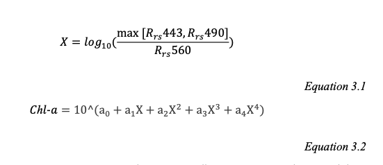
Where those a coefficients come from NASA Algorithms. Those three wavelengths correspond to the coastal band, the green band, and the blue band.
The second method is a bit simpler. It’s called the Chlorophyll Absorption Ratio Index (CARI).
 Let’s see how simple it is
to make these work for us!
More Resources
Chlorophyll A algorithms and NASA Earthdata.
O’Reilly, J. E., & Werdell, P. J. (2019). Chlorophyll algorithms for ocean color sensors-OC4, OC5 & OC6. https://doi.org/10.1016/j.rse.2019.04.021
Load Libraries and Pre-Process the Data

For this episode, we will use the Landsat scene from 2023 and the
seagrass beds from Casco Bay in 2022 (we’ll assume they’re close enough
to 2023). Let’s start by loading terra, sf,
and ggplot2.
R
library(terra)
library(sf)
library(ggplot2)
library(tidyterra)
Next, let’s load our two different data sources. We will load the rasters into one stack for ease of use. We will also load the Casco AOI and Maine State borders for use in cropping and masking down to just water.
R
# ACOLITE corrected Rrs - note, just the tifs, as the png is a thumbnail
landsat_files <- list.files(
  "data/landsat_casco/L8_OLI_2023_02_07_15_27_04_012030_L2R/",
           pattern = "tif",
           full.names = TRUE)

# Load all of the tifs
landsat_layers <- rast(landsat_files)

# give the layers better names
names(landsat_layers) <- c("blue_443", "blue_483", "green_561")

# load our shapefile
seagrass_casco_2022 <- st_read(
  "data/maine_gov_seagrass/MaineDEP_Casco_Bay_Seagrass_2022/MaineDEP_Casco_Bay_Seagrass_2022.shp")

# Load files for processing
aoi_boundary_casco <- st_read(
  "data/maine_gov_maps/casco_aoi/casco_bay_aoi.shp")

maine_borders <- st_read(
  "data/maine_gov_maps/Maine_State_Boundary_Polygon_Feature/Maine_State_Boundary_Polygon_Feature.shp")
R
describe(sources(landsat_layers))
OUTPUT
  [1] "Driver: GTiff/GeoTIFF"
  [2] "Files: /home/runner/work/r-raster-vector-geospatial/r-raster-vector-geospatial/site/built/data/landsat_casco/L8_OLI_2023_02_07_15_27_04_012030_L2R/L8_OLI_2023_02_07_15_27_04_012030_L2W_Rrs_443.tif"
  [3] "Size is 7891, 8001"
  [4] "Coordinate System is:"
  [5] "PROJCRS[\"WGS 84 / UTM zone 19N\","
  [6] "    BASEGEOGCRS[\"WGS 84\","
  [7] "        DATUM[\"World Geodetic System 1984\","
  [8] "            ELLIPSOID[\"WGS 84\",6378137,298.257223563,"
  [9] "                LENGTHUNIT[\"metre\",1]]],"
 [10] "        PRIMEM[\"Greenwich\",0,"
 [11] "            ANGLEUNIT[\"degree\",0.0174532925199433]],"
 [12] "        ID[\"EPSG\",4326]],"
 [13] "    CONVERSION[\"UTM zone 19N\","
 [14] "        METHOD[\"Transverse Mercator\","
 [15] "            ID[\"EPSG\",9807]],"
 [16] "        PARAMETER[\"Latitude of natural origin\",0,"
 [17] "            ANGLEUNIT[\"degree\",0.0174532925199433],"
 [18] "            ID[\"EPSG\",8801]],"
 [19] "        PARAMETER[\"Longitude of natural origin\",-69,"
 [20] "            ANGLEUNIT[\"degree\",0.0174532925199433],"
 [21] "            ID[\"EPSG\",8802]],"
 [22] "        PARAMETER[\"Scale factor at natural origin\",0.9996,"
 [23] "            SCALEUNIT[\"unity\",1],"
 [24] "            ID[\"EPSG\",8805]],"
 [25] "        PARAMETER[\"False easting\",500000,"
 [26] "            LENGTHUNIT[\"metre\",1],"
 [27] "            ID[\"EPSG\",8806]],"
 [28] "        PARAMETER[\"False northing\",0,"
 [29] "            LENGTHUNIT[\"metre\",1],"
 [30] "            ID[\"EPSG\",8807]]],"
 [31] "    CS[Cartesian,2],"
 [32] "        AXIS[\"(E)\",east,"
 [33] "            ORDER[1],"
 [34] "            LENGTHUNIT[\"metre\",1]],"
 [35] "        AXIS[\"(N)\",north,"
 [36] "            ORDER[2],"
 [37] "            LENGTHUNIT[\"metre\",1]],"
 [38] "    USAGE["
 [39] "        SCOPE[\"Engineering survey, topographic mapping.\"],"
 [40] "        AREA[\"Between 72°W and 66°W, northern hemisphere between equator and 84°N, onshore and offshore. Aruba. Bahamas. Brazil. Canada - New Brunswick (NB); Labrador; Nunavut; Nova Scotia (NS); Quebec. Colombia. Dominican Republic. Greenland. Netherlands Antilles. Puerto Rico. Turks and Caicos Islands. United States. Venezuela.\"],"
 [41] "        BBOX[0,-72,84,-66]],"
 [42] "    ID[\"EPSG\",32619]]"
 [43] "Data axis to CRS axis mapping: 1,2"
 [44] "Origin = (227370.000000000000000,4902630.000000000000000)"
 [45] "Pixel Size = (30.000000000000000,-30.000000000000000)"
 [46] "Metadata:"
 [47] "  AREA_OR_POINT=Area"
 [48] "  NC_GLOBAL#1_f0=19142.12138055756"
 [49] "  NC_GLOBAL#1_name=443"
 [50] "  NC_GLOBAL#1_wave=442.9823263713434"
 [51] "  NC_GLOBAL#2_f0=20166.79005236374"
 [52] "  NC_GLOBAL#2_name=483"
 [53] "  NC_GLOBAL#2_wave=482.5891954914198"
 [54] "  NC_GLOBAL#3_f0=18674.24059678011"
 [55] "  NC_GLOBAL#3_name=561"
 [56] "  NC_GLOBAL#3_wave=561.3326591091178"
 [57] "  NC_GLOBAL#4_f0=15649.95869773406"
 [58] "  NC_GLOBAL#4_name=655"
 [59] "  NC_GLOBAL#4_wave=654.606047604168"
 [60] "  NC_GLOBAL#5_f0=9484.951897185036"
 [61] "  NC_GLOBAL#5_name=865"
 [62] "  NC_GLOBAL#5_wave=864.5710906521408"
 [63] "  NC_GLOBAL#6_f0=2387.412329710507"
 [64] "  NC_GLOBAL#6_name=1609"
 [65] "  NC_GLOBAL#6_wave=1609.090443719705"
 [66] "  NC_GLOBAL#7_f0=814.198506038592"
 [67] "  NC_GLOBAL#7_name=2201"
 [68] "  NC_GLOBAL#7_wave=2201.248051984069"
 [69] "  NC_GLOBAL#8_f0=17580.89139262524"
 [70] "  NC_GLOBAL#8_name=592"
 [71] "  NC_GLOBAL#8_wave=591.6668530611159"
 [72] "  NC_GLOBAL#9_f0=3585.513285112"
 [73] "  NC_GLOBAL#9_name=1373"
 [74] "  NC_GLOBAL#9_wave=1373.476437717959"
 [75] "  NC_GLOBAL#acolite_file_type=L2R"
 [76] "  NC_GLOBAL#acolite_version=Generic GitHub Clone c2023-10-25T11:06:29"
 [77] "  NC_GLOBAL#acstar3_ex=3"
 [78] "  NC_GLOBAL#acstar3_fit_all_bands=True"
 [79] "  NC_GLOBAL#acstar3_mask_edges=True"
 [80] "  NC_GLOBAL#acstar3_max_wavelength=720"
 [81] "  NC_GLOBAL#acstar3_method=iter"
 [82] "  NC_GLOBAL#acstar3_psf_raster=False"
 [83] "  NC_GLOBAL#acstar3_write_rhoa=True"
 [84] "  NC_GLOBAL#acstar3_write_rhoe=True"
 [85] "  NC_GLOBAL#acstar3_write_rhosu=True"
 [86] "  NC_GLOBAL#add_band_name=False"
 [87] "  NC_GLOBAL#adjacency_correction=False"
 [88] "  NC_GLOBAL#adjacency_method=acstar3"
 [89] "  NC_GLOBAL#aerosol_correction=dark_spectrum"
 [90] "  NC_GLOBAL#ancillary_data=True"
 [91] "  NC_GLOBAL#ancillary_type=GMAO_MERRA2_MET"
 [92] "  NC_GLOBAL#atmospheric_correction=True"
 [93] "  NC_GLOBAL#auto_grouping=rhot:rhorc:rhos:rhow:Rrs:Lt"
 [94] "  NC_GLOBAL#blackfill_max=1.0"
 [95] "  NC_GLOBAL#blackfill_skip=True"
 [96] "  NC_GLOBAL#blackfill_wave=1600"
 [97] "  NC_GLOBAL#chris_interband_calibration=False"
 [98] "  NC_GLOBAL#chris_noise_reduction=True"
 [99] "  NC_GLOBAL#cirrus_correction=False"
[100] "  NC_GLOBAL#cirrus_g_swir=0.5"
[101] "  NC_GLOBAL#cirrus_g_vnir=1.0"
[102] "  NC_GLOBAL#cirrus_range={1350,1390}"
[103] "  NC_GLOBAL#clear_scratch=True"
[104] "  NC_GLOBAL#compute_contrabands=True"
[105] "  NC_GLOBAL#contact=Quinten Vanhellemont"
[106] "  NC_GLOBAL#Conventions=CF-1.7"
[107] "  NC_GLOBAL#copy_datasets={lon,lat,sza,vza,raa,rhot_*}"
[108] "  NC_GLOBAL#data_dimensions={8001,7891}"
[109] "  NC_GLOBAL#data_elements=63135891"
[110] "  NC_GLOBAL#delete_acolite_output_directory=False"
[111] "  NC_GLOBAL#delete_acolite_run_text_files=False"
[112] "  NC_GLOBAL#delete_extracted_input=False"
[113] "  NC_GLOBAL#dem_pressure=False"
[114] "  NC_GLOBAL#dem_pressure_percentile=25"
[115] "  NC_GLOBAL#dem_pressure_resolved=True"
[116] "  NC_GLOBAL#dem_pressure_write=False"
[117] "  NC_GLOBAL#dem_source=copernicus30"
[118] "  NC_GLOBAL#desis_mask_ql=True"
[119] "  NC_GLOBAL#dsf_allow_lut_boundaries=False"
[120] "  NC_GLOBAL#dsf_aot_compute=min"
[121] "  NC_GLOBAL#dsf_aot_estimate=tiled"
[122] "  NC_GLOBAL#dsf_aot_fillnan=True"
[123] "  NC_GLOBAL#dsf_aot_most_common_model=True"
[124] "  NC_GLOBAL#dsf_filter_aot=False"
[125] "  NC_GLOBAL#dsf_filter_box={10,10}"
[126] "  NC_GLOBAL#dsf_filter_percentile=50"
[127] "  NC_GLOBAL#dsf_filter_rhot=False"
[128] "  NC_GLOBAL#dsf_fixed_lut=ACOLITE-LUT-202110-MOD2"
[129] "  NC_GLOBAL#dsf_intercept_pixels=200"
[130] "  NC_GLOBAL#dsf_interface_lut=ACOLITE-RSKY-202102-82W"
[131] "  NC_GLOBAL#dsf_interface_option=default"
[132] "  NC_GLOBAL#dsf_interface_reflectance=False"
[133] "  NC_GLOBAL#dsf_max_tile_aot=1.2"
[134] "  NC_GLOBAL#dsf_minimum_segment_size=1"
[135] "  NC_GLOBAL#dsf_min_tile_aot=0.01"
[136] "  NC_GLOBAL#dsf_min_tile_cover=0.1"
[137] "  NC_GLOBAL#dsf_model_selection=min_drmsd"
[138] "  NC_GLOBAL#dsf_nbands=2"
[139] "  NC_GLOBAL#dsf_nbands_fit=2"
[140] "  NC_GLOBAL#dsf_percentile=1.0"
[141] "  NC_GLOBAL#dsf_residual_glint_correction=False"
[142] "  NC_GLOBAL#dsf_residual_glint_correction_method=default"
[143] "  NC_GLOBAL#dsf_residual_glint_wave_range={1500,2400}"
[144] "  NC_GLOBAL#dsf_smooth_aot=False"
[145] "  NC_GLOBAL#dsf_smooth_box={10,10}"
[146] "  NC_GLOBAL#dsf_spectrum_option=intercept"
[147] "  NC_GLOBAL#dsf_tile_dimensions={200,200}"
[148] "  NC_GLOBAL#dsf_tile_interp_method=linear"
[149] "  NC_GLOBAL#dsf_tile_smoothing=True"
[150] "  NC_GLOBAL#dsf_tile_smoothing_kernel_size=3"
[151] "  NC_GLOBAL#dsf_wave_range={400,2500}"
[152] "  NC_GLOBAL#dsf_write_aot_550=False"
[153] "  NC_GLOBAL#dsf_write_tiled_parameters=False"
[154] "  NC_GLOBAL#eminet_fill=True"
[155] "  NC_GLOBAL#eminet_fill_dilate=False"
[156] "  NC_GLOBAL#eminet_model_version=20220809"
[157] "  NC_GLOBAL#eminet_netname=Net2"
[158] "  NC_GLOBAL#eminet_water_fill=True"
[159] "  NC_GLOBAL#eminet_water_threshold=0.0215"
[160] "  NC_GLOBAL#export_cloud_optimized_geotiff=False"
[161] "  NC_GLOBAL#export_geotiff_coordinates=False"
[162] "  NC_GLOBAL#exp_alpha_weighted=True"
[163] "  NC_GLOBAL#exp_fixed_aerosol_reflectance=True"
[164] "  NC_GLOBAL#exp_fixed_aerosol_reflectance_percentile=5"
[165] "  NC_GLOBAL#exp_fixed_epsilon=True"
[166] "  NC_GLOBAL#exp_fixed_epsilon_percentile=50"
[167] "  NC_GLOBAL#exp_output_intermediate=False"
[168] "  NC_GLOBAL#exp_swir_threshold=0.0215"
[169] "  NC_GLOBAL#exp_wave1=1600"
[170] "  NC_GLOBAL#exp_wave2=2200"
[171] "  NC_GLOBAL#extend_region=False"
[172] "  NC_GLOBAL#flag_exponent_cirrus=1"
[173] "  NC_GLOBAL#flag_exponent_mixed=5"
[174] "  NC_GLOBAL#flag_exponent_negative=3"
[175] "  NC_GLOBAL#flag_exponent_outofscene=4"
[176] "  NC_GLOBAL#flag_exponent_swir=0"
[177] "  NC_GLOBAL#flag_exponent_toa=2"
[178] "  NC_GLOBAL#gains=False"
[179] "  NC_GLOBAL#gains_parameter=radiance"
[180] "  NC_GLOBAL#gains_toa={1,1,1,1,1,1,1,1,1}"
[181] "  NC_GLOBAL#ged_fill=True"
[182] "  NC_GLOBAL#generated_by=ACOLITE"
[183] "  NC_GLOBAL#generated_on=2024-01-09 13:09:08 PST"
[184] "  NC_GLOBAL#geometry_fixed_footprint=False"
[185] "  NC_GLOBAL#geometry_override=False"
[186] "  NC_GLOBAL#geometry_per_band=False"
[187] "  NC_GLOBAL#geometry_res=60"
[188] "  NC_GLOBAL#geometry_type=grids_footprint"
[189] "  NC_GLOBAL#gf_reproject_to_utm=False"
[190] "  NC_GLOBAL#glint_mask_rhos_threshold=0.05"
[191] "  NC_GLOBAL#glint_mask_rhos_wave=1600"
[192] "  NC_GLOBAL#glint_write_rhog_all=False"
[193] "  NC_GLOBAL#glint_write_rhog_ref=False"
[194] "  NC_GLOBAL#global_dims={8001,7891}"
[195] "  NC_GLOBAL#inputfile=/Users/Meredith/Library/CloudStorage/GoogleDrive-meredith.mcpherson@umb.edu/My Drive/UMB/acolite_for_Jarrett/L1_LC08_L1TP_012030_20230207_20230217_02_T1"
[196] "  NC_GLOBAL#isodate=2023-02-07T15:27:04.4876930Z"
[197] "  NC_GLOBAL#K1_CONSTANT_BAND_10=774.8853"
[198] "  NC_GLOBAL#K1_CONSTANT_BAND_11=480.8883"
[199] "  NC_GLOBAL#K2_CONSTANT_BAND_10=1321.0789"
[200] "  NC_GLOBAL#K2_CONSTANT_BAND_11=1201.1442"
[201] "  NC_GLOBAL#l1r_crop=False"
[202] "  NC_GLOBAL#l1r_delete_netcdf=False"
[203] "  NC_GLOBAL#l1r_export_geotiff=False"
[204] "  NC_GLOBAL#l1r_export_geotiff_rgb=False"
[205] "  NC_GLOBAL#l2r_delete_netcdf=False"
[206] "  NC_GLOBAL#l2r_export_geotiff=True"
[207] "  NC_GLOBAL#l2r_export_geotiff_rgb=False"
[208] "  NC_GLOBAL#l2r_pans_delete_netcdf=False"
[209] "  NC_GLOBAL#l2t_delete_netcdf=False"
[210] "  NC_GLOBAL#l2t_export_geotiff=False"
[211] "  NC_GLOBAL#l2w_data_in_memory=False"
[212] "  NC_GLOBAL#l2w_delete_netcdf=False"
[213] "  NC_GLOBAL#l2w_export_geotiff=True"
[214] "  NC_GLOBAL#l2w_mask=True"
[215] "  NC_GLOBAL#l2w_mask_cirrus=True"
[216] "  NC_GLOBAL#l2w_mask_cirrus_threshold=0.005"
[217] "  NC_GLOBAL#l2w_mask_cirrus_wave=1373"
[218] "  NC_GLOBAL#l2w_mask_high_toa=True"
[219] "  NC_GLOBAL#l2w_mask_high_toa_threshold=0.3"
[220] "  NC_GLOBAL#l2w_mask_high_toa_wave_range={400,2500}"
[221] "  NC_GLOBAL#l2w_mask_mixed=True"
[222] "  NC_GLOBAL#l2w_mask_negative_rhow=True"
[223] "  NC_GLOBAL#l2w_mask_negative_wave_range={400,900}"
[224] "  NC_GLOBAL#l2w_mask_smooth=True"
[225] "  NC_GLOBAL#l2w_mask_smooth_sigma=3"
[226] "  NC_GLOBAL#l2w_mask_threshold=0.0215"
[227] "  NC_GLOBAL#l2w_mask_water_parameters=True"
[228] "  NC_GLOBAL#l2w_mask_wave=1600"
[229] "  NC_GLOBAL#l2w_parameters={rhos_*,rhow_*,Rrs_*,l2w_export_geotiff=True,l2r_export_geotiff=True}"
[230] "  NC_GLOBAL#landsat_qa_bands={PIXEL,RADSAT,SATURATION}"
[231] "  NC_GLOBAL#landsat_qa_output=False"
[232] "  NC_GLOBAL#luts={ACOLITE-LUT-202110-MOD1,ACOLITE-LUT-202110-MOD2}"
[233] "  NC_GLOBAL#luts_pressures={500,750,1013,1100}"
[234] "  NC_GLOBAL#luts_reduce_dimensions=True"
[235] "  NC_GLOBAL#map_auto_range=False"
[236] "  NC_GLOBAL#map_auto_range_percentiles={1,99}"
[237] "  NC_GLOBAL#map_cartopy=False"
[238] "  NC_GLOBAL#map_colorbar=True"
[239] "  NC_GLOBAL#map_colorbar_orientation=vertical"
[240] "  NC_GLOBAL#map_default_colormap=viridis"
[241] "  NC_GLOBAL#map_dpi=300"
[242] "  NC_GLOBAL#map_ext=png"
[243] "  NC_GLOBAL#map_fill_color=LightGrey"
[244] "  NC_GLOBAL#map_fill_outrange=False"
[245] "  NC_GLOBAL#map_fontname=sans-serif"
[246] "  NC_GLOBAL#map_fontsize=12"
[247] "  NC_GLOBAL#map_gridline_color=white"
[248] "  NC_GLOBAL#map_l2w=True"
[249] "  NC_GLOBAL#map_mask=True"
[250] "  NC_GLOBAL#map_pcolormesh=False"
[251] "  NC_GLOBAL#map_projected=False"
[252] "  NC_GLOBAL#map_raster=False"
[253] "  NC_GLOBAL#map_scalebar=False"
[254] "  NC_GLOBAL#map_scalebar_color=Black"
[255] "  NC_GLOBAL#map_scalebar_max_fraction=0.33"
[256] "  NC_GLOBAL#map_scalebar_position=UL"
[257] "  NC_GLOBAL#map_title=True"
[258] "  NC_GLOBAL#map_usetex=False"
[259] "  NC_GLOBAL#map_xtick_rotation=0.0"
[260] "  NC_GLOBAL#map_ytick_rotation=0.0"
[261] "  NC_GLOBAL#merge_tiles=False"
[262] "  NC_GLOBAL#merge_zones=True"
[263] "  NC_GLOBAL#metadata_profile=beam"
[264] "  NC_GLOBAL#metadata_version=0.5"
[265] "  NC_GLOBAL#min_tgas_aot=0.85"
[266] "  NC_GLOBAL#min_tgas_rho=0.7"
[267] "  NC_GLOBAL#mus=0.4690880680561129"
[268] "  NC_GLOBAL#nechad_max_rhow_C_factor=0.5"
[269] "  NC_GLOBAL#nechad_range={600,900}"
[270] "  NC_GLOBAL#netcdf_compression=False"
[271] "  NC_GLOBAL#netcdf_compression_level=4"
[272] "  NC_GLOBAL#netcdf_discretisation=False"
[273] "  NC_GLOBAL#netcdf_projection=True"
[274] "  NC_GLOBAL#offsets=False"
[275] "  NC_GLOBAL#ofile=/Users/Meredith/Library/CloudStorage/GoogleDrive-meredith.mcpherson@umb.edu/My Drive/UMB/acolite_for_Jarrett/acolite_output/L8_OLI_2023_02_07_15_27_04_012030_L2W.nc"
[276] "  NC_GLOBAL#oname=L8_OLI_2023_02_07_15_27_04_012030"
[277] "  NC_GLOBAL#output=/Users/Meredith/Library/CloudStorage/GoogleDrive-meredith.mcpherson@umb.edu/My Drive/UMB/acolite_for_Jarrett/acolite_output"
[278] "  NC_GLOBAL#output_bt=False"
[279] "  NC_GLOBAL#output_geolocation=True"
[280] "  NC_GLOBAL#output_geometry=True"
[281] "  NC_GLOBAL#output_lt=False"
[282] "  NC_GLOBAL#output_projection=False"
[283] "  NC_GLOBAL#output_projection_epsilon=0.0"
[284] "  NC_GLOBAL#output_projection_filldistance=1"
[285] "  NC_GLOBAL#output_projection_fillnans=False"
[286] "  NC_GLOBAL#output_projection_metres=False"
[287] "  NC_GLOBAL#output_projection_neighbours=32"
[288] "  NC_GLOBAL#output_projection_radius=3"
[289] "  NC_GLOBAL#output_projection_resampling_method=bilinear"
[290] "  NC_GLOBAL#output_projection_resolution_align=True"
[291] "  NC_GLOBAL#output_rhorc=False"
[292] "  NC_GLOBAL#output_xy=False"
[293] "  NC_GLOBAL#pans=False"
[294] "  NC_GLOBAL#pans_bgr={480,560,655}"
[295] "  NC_GLOBAL#pans_export_geotiff_rgb=False"
[296] "  NC_GLOBAL#pans_method=panr"
[297] "  NC_GLOBAL#pans_output=rgb"
[298] "  NC_GLOBAL#pans_rgb_rhos=True"
[299] "  NC_GLOBAL#pans_rgb_rhot=True"
[300] "  NC_GLOBAL#pans_sensors={L7_ETM,L8_OLI,L9_OLI}"
[301] "  NC_GLOBAL#pan_dims={16002,15782}"
[302] "  NC_GLOBAL#pixel_size={30,-30}"
[303] "  NC_GLOBAL#planet_store_sr=False"
[304] "  NC_GLOBAL#pleiades_skip_pan=False"
[305] "  NC_GLOBAL#polygon_limit=True"
[306] "  NC_GLOBAL#polylakes=False"
[307] "  NC_GLOBAL#polylakes_database=worldlakes"
[308] "  NC_GLOBAL#pressure=1013.25"
[309] "  NC_GLOBAL#pressure_default=1013.25"
[310] "  NC_GLOBAL#prisma_output_pan=False"
[311] "  NC_GLOBAL#prisma_rhot_per_pixel_sza=True"
[312] "  NC_GLOBAL#prisma_store_l2c=False"
[313] "  NC_GLOBAL#prisma_store_l2c_separate_file=True"
[314] "  NC_GLOBAL#product_type=NetCDF"
[315] "  NC_GLOBAL#proj4_string=+proj=utm +zone=19 +datum=WGS84 +units=m +no_defs "
[316] "  NC_GLOBAL#projection_key=transverse_mercator"
[317] "  NC_GLOBAL#raa=39.14653566267489"
[318] "  NC_GLOBAL#radcor_bratio_option=percentile"
[319] "  NC_GLOBAL#radcor_bratio_percentile=1.0"
[320] "  NC_GLOBAL#radcor_expand_edge=True"
[321] "  NC_GLOBAL#radcor_expand_method=mirror"
[322] "  NC_GLOBAL#radcor_fft_stack=False"
[323] "  NC_GLOBAL#radcor_initial_aot=0.3"
[324] "  NC_GLOBAL#radcor_mask_edges=True"
[325] "  NC_GLOBAL#radcor_psf_complete_method=neighborhood"
[326] "  NC_GLOBAL#radcor_psf_radius=3.5"
[327] "  NC_GLOBAL#radcor_psf_rescale=False"
[328] "  NC_GLOBAL#radcor_write_rhoe=True"
[329] "  NC_GLOBAL#radcor_write_rhot=True"
[330] "  NC_GLOBAL#reproject_before_ac=False"
[331] "  NC_GLOBAL#reproject_inputfile=False"
[332] "  NC_GLOBAL#reproject_inputfile_dem=False"
[333] "  NC_GLOBAL#reproject_inputfile_force=False"
[334] "  NC_GLOBAL#reproject_outputs={L1R,L2R,L2W}"
[335] "  NC_GLOBAL#resolved_geometry=True"
[336] "  NC_GLOBAL#rgb_autoscale=False"
[337] "  NC_GLOBAL#rgb_autoscale_percentiles={5,95}"
[338] "  NC_GLOBAL#rgb_blue_wl=480"
[339] "  NC_GLOBAL#rgb_gamma={1,1,1}"
[340] "  NC_GLOBAL#rgb_green_wl=560"
[341] "  NC_GLOBAL#rgb_max={0.15,0.15,0.15}"
[342] "  NC_GLOBAL#rgb_min={0,0,0}"
[343] "  NC_GLOBAL#rgb_red_wl=650"
[344] "  NC_GLOBAL#rgb_rhorc=False"
[345] "  NC_GLOBAL#rgb_rhos=True"
[346] "  NC_GLOBAL#rgb_rhot=True"
[347] "  NC_GLOBAL#rgb_rhow=False"
[348] "  NC_GLOBAL#rgb_stretch=linear"
[349] "  NC_GLOBAL#runid=20240109_125219"
[350] "  NC_GLOBAL#s2_dilate_blackfill=False"
[351] "  NC_GLOBAL#s2_dilate_blackfill_iterations=2"
[352] "  NC_GLOBAL#s2_include_auxillary=False"
[353] "  NC_GLOBAL#s2_project_auxillary=True"
[354] "  NC_GLOBAL#s2_target_res=10"
[355] "  NC_GLOBAL#s2_write_dfoo=False"
[356] "  NC_GLOBAL#s2_write_saa=False"
[357] "  NC_GLOBAL#s2_write_vaa=False"
[358] "  NC_GLOBAL#saa=155.12723673"
[359] "  NC_GLOBAL#scene_dims={8001,7891}"
[360] "  NC_GLOBAL#scene_download=False"
[361] "  NC_GLOBAL#scene_pixel_size={30,-30}"
[362] "  NC_GLOBAL#scene_proj4_string=+proj=utm +zone=19 +datum=WGS84 +units=m +no_defs "
[363] "  NC_GLOBAL#scene_xrange={227385,464115}"
[364] "  NC_GLOBAL#scene_yrange={4902615,4662585}"
[365] "  NC_GLOBAL#scene_zone=19"
[366] "  NC_GLOBAL#sensor=L8_OLI"
[367] "  NC_GLOBAL#se_distance=0.9862333"
[368] "  NC_GLOBAL#slicing=False"
[369] "  NC_GLOBAL#smile_correction=True"
[370] "  NC_GLOBAL#smile_correction_tgas=True"
[371] "  NC_GLOBAL#solar_irradiance_reference=Coddington2021_1_0nm"
[372] "  NC_GLOBAL#sza=62.02488267"
[373] "  NC_GLOBAL#sza_limit=79.999"
[374] "  NC_GLOBAL#sza_limit_replace=False"
[375] "  NC_GLOBAL#tact_emissivity=water"
[376] "  NC_GLOBAL#tact_map=True"
[377] "  NC_GLOBAL#tact_output_atmosphere=False"
[378] "  NC_GLOBAL#tact_output_intermediate=False"
[379] "  NC_GLOBAL#tact_profile_source=era5"
[380] "  NC_GLOBAL#tact_range={3.5,14}"
[381] "  NC_GLOBAL#tact_reptran=medium"
[382] "  NC_GLOBAL#tact_run=False"
[383] "  NC_GLOBAL#thermal_bands={10,11}"
[384] "  NC_GLOBAL#thermal_sensor=L8_TIRS"
[385] "  NC_GLOBAL#tile_code=012030"
[386] "  NC_GLOBAL#uoz=0.3"
[387] "  NC_GLOBAL#uoz_default=0.3"
[388] "  NC_GLOBAL#use_gdal_merge_import=False"
[389] "  NC_GLOBAL#use_supplied_ancillary=True"
[390] "  NC_GLOBAL#use_tpg=True"
[391] "  NC_GLOBAL#uwv=1.5"
[392] "  NC_GLOBAL#uwv_default=1.5"
[393] "  NC_GLOBAL#vaa=194.2737723926749"
[394] "  NC_GLOBAL#verbosity=5"
[395] "  NC_GLOBAL#viirs_mask_immixed=True"
[396] "  NC_GLOBAL#viirs_mask_immixed_bands=I03/M10"
[397] "  NC_GLOBAL#viirs_mask_immixed_dif=True"
[398] "  NC_GLOBAL#viirs_mask_immixed_maxdif=0.002"
[399] "  NC_GLOBAL#viirs_mask_immixed_maxrat=0.2"
[400] "  NC_GLOBAL#viirs_mask_immixed_rat=False"
[401] "  NC_GLOBAL#viirs_mask_mband=True"
[402] "  NC_GLOBAL#viirs_option=img+mod"
[403] "  NC_GLOBAL#viirs_output_tir=True"
[404] "  NC_GLOBAL#viirs_output_tir_lt=False"
[405] "  NC_GLOBAL#viirs_quality_flags={4,8,512,1024,2048,4096}"
[406] "  NC_GLOBAL#viirs_scanline_projection=True"
[407] "  NC_GLOBAL#viirs_scanline_width=32"
[408] "  NC_GLOBAL#vza=0"
[409] "  NC_GLOBAL#vza_limit=71.999"
[410] "  NC_GLOBAL#vza_limit_replace=False"
[411] "  NC_GLOBAL#wind=2"
[412] "  NC_GLOBAL#wind_default=2"
[413] "  NC_GLOBAL#worldview_reproject=False"
[414] "  NC_GLOBAL#worldview_reproject_method=nearest"
[415] "  NC_GLOBAL#worldview_reproject_resolution=2"
[416] "  NC_GLOBAL#wrs_path=12"
[417] "  NC_GLOBAL#wrs_row=30"
[418] "  NC_GLOBAL#xdim=7891"
[419] "  NC_GLOBAL#xrange={227370,464100}"
[420] "  NC_GLOBAL#ydim=8001"
[421] "  NC_GLOBAL#yrange={4902630,4662600}"
[422] "  NC_GLOBAL#zone=19"
[423] "  Rrs_443#dataset=rhos"
[424] "  Rrs_443#grid_mapping=transverse_mercator"
[425] "  Rrs_443#long_name=Surface reflectance"
[426] "  Rrs_443#parameter=Rrs_443"
[427] "  Rrs_443#rhos_ds=rhos_443"
[428] "  Rrs_443#rhot_ds=rhot_443"
[429] "  Rrs_443#standard_name=surface_bidirectional_reflectance"
[430] "  Rrs_443#tt_ch4=1"
[431] "  Rrs_443#tt_co2=1"
[432] "  Rrs_443#tt_gas=0.9972927231155655"
[433] "  Rrs_443#tt_h2o=1"
[434] "  Rrs_443#tt_n2o=1"
[435] "  Rrs_443#tt_o2=1"
[436] "  Rrs_443#tt_o3=0.9972927231155655"
[437] "  Rrs_443#units=1"
[438] "  Rrs_443#wavelength=442.9822110780657"
[439] "  Rrs_443#wave_mu=0.4429822110780657"
[440] "  Rrs_443#wave_name=443"
[441] "  Rrs_443#wave_nm=442.9822110780657"
[442] "  transverse_mercator#crs_wkt=PROJCRS[\"unknown\",BASEGEOGCRS[\"unknown\",DATUM[\"World Geodetic System 1984\",ELLIPSOID[\"WGS 84\",6378137,298.257223563,LENGTHUNIT[\"metre\",1]],ID[\"EPSG\",6326]],PRIMEM[\"Greenwich\",0,ANGLEUNIT[\"degree\",0.0174532925199433],ID[\"EPSG\",8901]]],CONVERSION[\"UTM zone 19N\",METHOD[\"Transverse Mercator\",ID[\"EPSG\",9807]],PARAMETER[\"Latitude of natural origin\",0,ANGLEUNIT[\"degree\",0.0174532925199433],ID[\"EPSG\",8801]],PARAMETER[\"Longitude of natural origin\",-69,ANGLEUNIT[\"degree\",0.0174532925199433],ID[\"EPSG\",8802]],PARAMETER[\"Scale factor at natural origin\",0.9996,SCALEUNIT[\"unity\",1],ID[\"EPSG\",8805]],PARAMETER[\"False easting\",500000,LENGTHUNIT[\"metre\",1],ID[\"EPSG\",8806]],PARAMETER[\"False northing\",0,LENGTHUNIT[\"metre\",1],ID[\"EPSG\",8807]],ID[\"EPSG\",16019]],CS[Cartesian,2],AXIS[\"(E)\",east,ORDER[1],LENGTHUNIT[\"metre\",1,ID[\"EPSG\",9001]]],AXIS[\"(N)\",north,ORDER[2],LENGTHUNIT[\"metre\",1,ID[\"EPSG\",9001]]]]"
[443] "  transverse_mercator#false_easting=500000"
[444] "  transverse_mercator#false_northing=0"
[445] "  transverse_mercator#geographic_crs_name=unknown"
[446] "  transverse_mercator#grid_mapping_name=transverse_mercator"
[447] "  transverse_mercator#horizontal_datum_name=World Geodetic System 1984"
[448] "  transverse_mercator#inverse_flattening=298.257223563"
[449] "  transverse_mercator#latitude_of_projection_origin=0"
[450] "  transverse_mercator#longitude_of_central_meridian=-69"
[451] "  transverse_mercator#longitude_of_prime_meridian=0"
[452] "  transverse_mercator#prime_meridian_name=Greenwich"
[453] "  transverse_mercator#projected_crs_name=unknown"
[454] "  transverse_mercator#reference_ellipsoid_name=WGS 84"
[455] "  transverse_mercator#scale_factor_at_central_meridian=0.9996"
[456] "  transverse_mercator#semi_major_axis=6378137"
[457] "  transverse_mercator#semi_minor_axis=6356752.314245179"
[458] "  x#long_name=x coordinate of projection"
[459] "  x#standard_name=projection_x_coordinate"
[460] "  x#units=m"
[461] "  y#long_name=y coordinate of projection"
[462] "  y#standard_name=projection_y_coordinate"
[463] "  y#units=m"
[464] "Image Structure Metadata:"
[465] "  INTERLEAVE=BAND"
[466] "Corner Coordinates:"
[467] "Upper Left  (  227370.000, 4902630.000) ( 72d24'48.22\"W, 44d13'33.20\"N)"
[468] "Lower Left  (  227370.000, 4662600.000) ( 72d17'42.95\"W, 42d 4' 5.38\"N)"
[469] "Upper Right (  464100.000, 4902630.000) ( 69d26'59.52\"W, 44d16'33.71\"N)"
[470] "Lower Right (  464100.000, 4662600.000) ( 69d26' 3.35\"W, 42d 6'52.84\"N)"
[471] "Center      (  345735.000, 4782615.000) ( 70d53'53.42\"W, 43d10'50.02\"N)"
[472] "Band 1 Block=7891x1 Type=Float32, ColorInterp=Gray"
[473] "  NoData Value=nan"
[474] "  Unit Type: 1"
[475] "  Metadata:"
[476] "    dataset=rhos"
[477] "    grid_mapping=transverse_mercator"
[478] "    long_name=Surface reflectance"
[479] "    NETCDF_VARNAME=Rrs_443"
[480] "    parameter=Rrs_443"
[481] "    rhos_ds=rhos_443"
[482] "    rhot_ds=rhot_443"
[483] "    standard_name=surface_bidirectional_reflectance"
[484] "    tt_ch4=1"
[485] "    tt_co2=1"
[486] "    tt_gas=0.9972927231155655"
[487] "    tt_h2o=1"
[488] "    tt_n2o=1"
[489] "    tt_o2=1"
[490] "    tt_o3=0.9972927231155655"
[491] "    units=1"
[492] "    wavelength=442.9822110780657"
[493] "    wave_mu=0.4429822110780657"
[494] "    wave_name=443"
[495] "    wave_nm=442.9822110780657"
R
seagrass_casco_2022
OUTPUT
Simple feature collection with 622 features and 15 fields
Geometry type: POLYGON
Dimension:     XY
Bounding box:  xmin: -70.24464 ymin: 43.57213 xmax: -69.84399 ymax: 43.93221
Geodetic CRS:  WGS 84
First 10 features:
   OBJECTID Id Name       Acres   Hectares Orth_Cover Cover_Pct Field_Ver
1         1  1   01  0.04456005 0.01803281          1      0-10         Y
2         2  4   02  0.06076669 0.02459141          3     40-70         Y
3         3  6   03  2.56218247 1.03687846          3     40-70         Y
4         4  8   05  0.71816162 0.29062970          3     40-70         Y
5         5  9   06  0.01815022 0.00734513          3     40-70         Y
6         6 10   07  0.33051475 0.13375458          3     40-70         Y
7         7 11   08  0.08088664 0.03273366          1      0-10         Y
8         8 13   09  0.66689055 0.26988103          1      0-10         Y
9         9 14   10  0.03080650 0.01246695          3     40-70         Y
10       10 15   11 12.54074080 5.07505774          4    70-100         Y
   Video_YN                          Video Comment        Species
1         Y                            A03    <NA> Zostera marina
2         Y                            A04    <NA> Zostera marina
3         Y                            A05    <NA> Zostera marina
4         Y                            A07    <NA> Zostera marina
5         Y                            A08    <NA> Zostera marina
6         Y                            A09    <NA> Zostera marina
7         Y                            A10    <NA> Zostera marina
8         Y                            A11    <NA> Zostera marina
9         Y                            A12    <NA> Zostera marina
10        Y A14, A15, A16, A17, SP07, SP08    <NA> Zostera marina
                                 GlobalID  ShapeSTAre ShapeSTLen
1  {7CAB9D54-4BF9-4B91-94D6-4F0EA4AD53C1}   180.32842  102.57257
2  {D5396F39-D508-45CB-BFE0-13A506D4E94C}   245.91500   84.35420
3  {3C1ED4DC-6580-4CAC-9499-32D445019068} 10368.78375  719.04025
4  {6C1395B8-F532-46C6-AFBA-23B14C2F2E02}  2906.29561  315.88722
5  {EDEDAFA1-8605-4FAC-910F-E6E864F51209}    73.45108   34.00204
6  {820DE3B5-BA6E-4415-A110-95F9F94A4F1C}  1337.54527  165.98655
7  {E4E2A155-7B1C-46C3-94B5-6D0E58B1FEBB}   327.33664  112.52478
8  {C7FEF8AC-9BA7-429C-A45B-270E836FBBA1}  2698.81099  295.01388
9  {356C58A4-DB72-445F-83DA-1035C8EAE917}   124.66947   43.47523
10 {C797140E-F9CB-4EA0-9D7C-FBEA50FE9EB2} 50750.58217 1949.02908
                         geometry
1  POLYGON ((-70.20081 43.5722...
2  POLYGON ((-70.20228 43.5869...
3  POLYGON ((-70.20858 43.5909...
4  POLYGON ((-70.21488 43.5924...
5  POLYGON ((-70.21499 43.5931...
6  POLYGON ((-70.21582 43.5963...
7  POLYGON ((-70.21618 43.5964...
8  POLYGON ((-70.21641 43.5971...
9  POLYGON ((-70.21498 43.6063...
10 POLYGON ((-70.22445 43.6425...
Different in CRS and extent. We will have to project and crop.
So, we have to get Landsat into the same CRS as our Maine data. We will then have to crop it down to the Casco region. This is actually one of those cases where it will be faster to reproject the vectors than the raster for the cropping.
R
aoi_boundary_casco_projected <- st_transform(aoi_boundary_casco,
                                             crs(landsat_layers))

landsat_layers_casco <- crop(landsat_layers,
                             aoi_boundary_casco_projected)

landsat_layers_casco <- project(landsat_layers_casco,
                                crs(seagrass_casco_2022))
Masking Out Land with a Vector
Let’s see what we have after the cropping.
R
ggplot() +
  geom_spatraster(data = landsat_layers_casco) +
  facet_wrap(~lyr) +
  scale_fill_distiller(palette = "Greys")
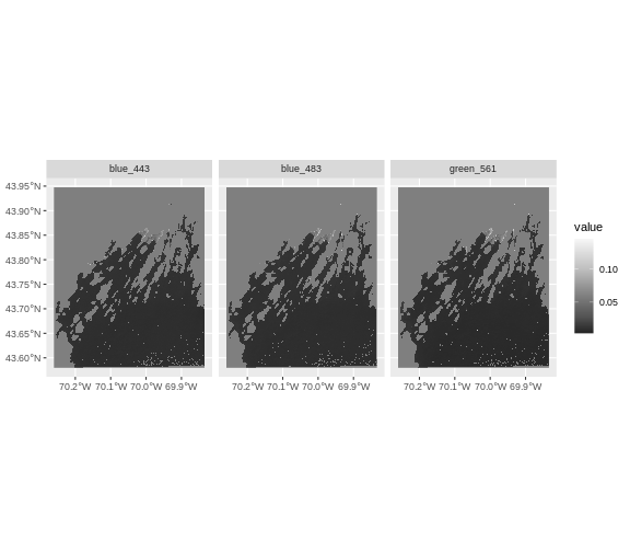
This is neat, but…… it’s dominated by the land. We want to mask the
land. Otherwise, the signal is going to be dominated by land and not
sea. Fortunately, we can use the coastline of the state from the maine
shapefile with mask(). By default, mask keeps what is IN
polygons. So we will need to use the argument
inverse = TRUE. We also need our coastline to have the same
extent as our raster, so, we’ll need to crop it first.
We will also recrop to the AOI again, as our previous crop leaves some cruft around the edges.
R
casco_coastline <- st_crop(maine_borders |> st_make_valid(),
                           aoi_boundary_casco)

# mask and crop
landsat_layers_casco_bay <- mask(landsat_layers_casco,
                                 casco_coastline,
                                 inverse = TRUE) |>
  crop(aoi_boundary_casco)
Did it blend?
R
ggplot() +
  geom_spatraster(data = landsat_layers_casco_bay ) +
  facet_wrap(~lyr) +
  scale_fill_distiller(palette = "Greys", na.value = NA)
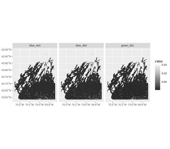
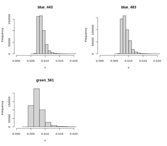
This looks great. There are still some really really high and low
values. We might want to figure out a threshold for clamping. Looking at
the histogram below, something like 0.02 for the upper seems reasonable.
We will use values=FALSE to just remove very high values
and make them NA.
R
# what do things look like?
hist(landsat_layers_casco_bay, breaks = 100, xlim = c(0,0.02))
R
#we include lower and upper for good measure
landsat_layers_casco_bay <- clamp(landsat_layers_casco_bay,
                                   lower = 0,
                                   upper = 0.02,
                                   value = FALSE)
Replot it, and, wow, you can really start to see some variability
Two Ways to Perform Raster Calculations
We can calculate with rasters in two different ways:
- by directly using the rasters in R using raster math
or for more efficient processing - particularly if our rasters are large and/or the calculations we are performing are complex:
- using the
lapp()function.
Raster Math & CARI
We can perform raster calculations by subtracting (or adding, multiplying, etc) two rasters. In the geospatial world, we call this “raster math”.
Let’s calculate (green - blue)/(green + blue) to get our CARI score.
After doing this, let’s plot with ggplot.
R
casco_cari <- (landsat_layers_casco_bay$green_561 - landsat_layers_casco_bay$blue_483) /
  (landsat_layers_casco_bay$green_561 + landsat_layers_casco_bay$blue_483)

names(casco_cari) <- "CARI"

ggplot() +
  geom_spatraster(data = casco_cari) +
  scale_fill_viridis_c() +
  labs(fill = "CARI")
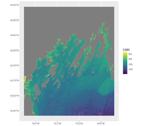
Let’s have a look at the distribution of values in our newly created CARI Model (CHM).
R
hist(casco_cari,
     maxcell = ncell(casco_cari))
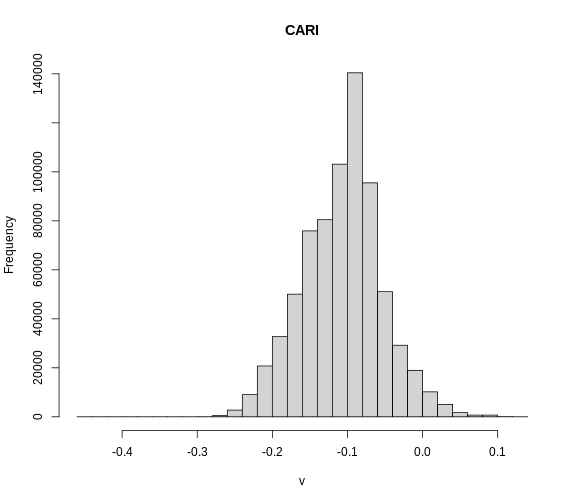
We are definitely starting to see some coastal features here, although whether it is chlorophyll or just coastal runoff is unclear.
Challenge: Explore CHM Raster Values
It’s often a good idea to explore the range of values in a raster dataset just like we might explore a dataset that we collected in the field. Or the spatial distribution to see if it lines up with expectations.
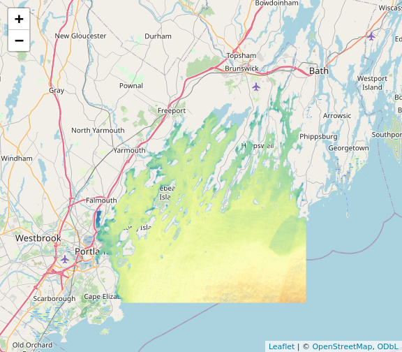
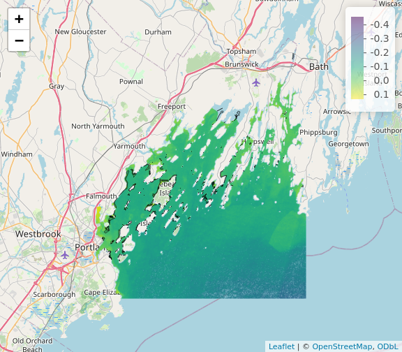
Zoom in on an island (Mackworth if you like). What does the spatial distribution look like? Use
ggplot2orleaflet.Overlay the seagrass bed shapefile. What do you see?
- Zooming in, some of the highest values are close to shorelines.
R
library(leaflet)

leaflet() |>
  addTiles() |>
  addRasterImage(x = casco_cari)
R
library(leaflet)

pal <- colorNumeric("viridis", values(casco_cari), na.color = NA)

leaflet() |>
  addTiles() |>
  addRasterImage(x = casco_cari,
                 colors = pal) |>
  addPolygons(data = seagrass_casco_2022,
               color = "black",
               weight = 1) |>
  addLegend(pal = pal, values = values(casco_cari))
Efficient Raster Calculations
Raster math, like we just did, is an appropriate approach to raster calculations if:
- The rasters we are using are small in size.
- The calculations we are performing are simple.
However, raster math is a less efficient approach as computation becomes more complex or as file sizes become large.
The lapp() function takes two or more rasters and
applies a function to them using efficient processing methods. The
syntax is
outputRaster <- lapp(x, fun=functionName)
In which raster can be either a SpatRaster or a SpatRasterDataset
which is an object that holds rasters. See help(sds).
If you have a raster, stack, you can instead use
app()
outputRaster <- app(x, fun=functionName)
Let’s perform the chla calculation that we calculated above using
raster math, using the app() function.
Data Tip
A custom function consists of a defined set of commands performed on
a input object. Custom functions are particularly useful for tasks that
need to be repeated over and over in the code. A simplified syntax for
writing a custom function in R is:
function_name <- function(variable1, variable2) { WhatYouWantDone, WhatToReturn}
R
get_chl <- function(rast_stack){

  #eqn 3.1
  x <- log10(max(rast_stack[1], rast_stack[2])/rast_stack[3])

  #eqn 3.2
  10^(0.30963 + -2.40052*x + 1.28932*x^2 + 0.52802*x^3 + -1.33825*x^4)
  }

casco_chla <- app(landsat_layers_casco_bay,
                    fun = get_chl)

names(casco_chla) <- "chla"
Now we can plot the CHLa:
R
 ggplot() +
   geom_spatraster(data = casco_chla) +
  scale_fill_viridis_c() +
  labs(fill = "Chl a")
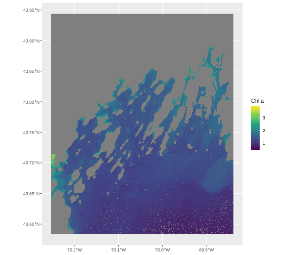
How do the plots of the CHM created with manual raster math and the
lapp() function compare?
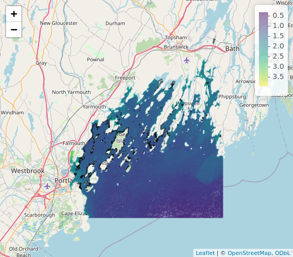
Qualitatively, they look about the same!
R
library(leaflet)

pal_chl <- colorNumeric("viridis", values(casco_chla), na.color = NA)

leaflet() |>
  addTiles() |>
  addRasterImage(x = casco_chla,
                 colors = pal_chl) |>
  addPolygons(data = seagrass_casco_2022,
               color = "black",
               weight = 2,
              fill = NA) |>
  addLegend(pal = pal_chl, values = values(casco_chla))
Export a GeoTIFF
Now that we’ve created a new raster, let’s export the data as a
GeoTIFF file using the writeRaster() function.
When we write this raster object to a GeoTIFF file we’ll name it
casco_cari.tif. This name allows us to quickly remember
both what the data contains (CARI data) and for where (Casco bay). The
writeRaster() function by default writes the output file to
your working directory unless you specify a full file path.
We will specify the output format (“GTiff”), the no data value
NAflag = -9999. We will also tell R to overwrite any data
that is already in a file of the same name.
R
writeRaster(casco_cari, "data/casco_cari.tif",
            filetype="GTiff",
            overwrite=TRUE,
            NAflag=-9999)
writeRaster() Options
The function arguments that we used above include:
-
filetype: specify that the format will be
GTiffor GeoTIFF. - overwrite: If TRUE, R will overwrite any existing file with the same name in the specified directory. USE THIS SETTING WITH CAUTION!
-
NAflag: set the GeoTIFF tag for
NoDataValueto -9999, the National Ecological Observatory Network’s (NEON) standardNoDataValue.
