Content from Intro to Raster Data
Last updated on 2024-03-12 | Edit this page
Estimated time: 50 minutes
OUTPUT
phantomjs has been installed to /home/runner/binWARNING
Warning in
download.file("https://www.naturalearthdata.com/http//www.naturalearthdata.com/download/110m/physical/ne_110m_graticules_all.zip",
: cannot open URL
'https://www.naturalearthdata.com/http//www.naturalearthdata.com/download/110m/physical/ne_110m_graticules_all.zip':
HTTP status was '500 Internal Server Error'
ERROR
Error in download.file("https://www.naturalearthdata.com/http//www.naturalearthdata.com/download/110m/physical/ne_110m_graticules_all.zip", : cannot open URL 'https://www.naturalearthdata.com/http//www.naturalearthdata.com/download/110m/physical/ne_110m_graticules_all.zip'Overview
Questions
- What is a raster dataset?
- How do I work with and plot raster data in R?
- How can I handle missing or bad data values for a raster?
Objectives
- Describe the fundamental attributes of a raster dataset.
- Explore raster attributes and metadata using R.
- Import rasters into R using the
terrapackage. - Plot a raster file in R using the
ggplot2package. - Describe the difference between single- and multi-band rasters.
Things You’ll Need To Complete This Episode
See the lesson homepage for detailed information about the software, data, and other prerequisites you will need to work through the examples in this episode.
In this episode, we will introduce the fundamental principles, packages and metadata/raster attributes that are needed to work with raster data in R. We will discuss some of the core metadata elements that we need to understand to work with rasters in R, including CRS and resolution. We will also explore missing and bad data values as stored in a raster and how R handles these elements.
We will continue to work with the dplyr and
ggplot2 packages that were introduced in the Introduction
to R for Geospatial Data lesson. We will use two additional packages
in this episode to work with raster data - the terra and
sf packages. Make sure that you have these packages
loaded.
R
library(terra)
library(ggplot2)
library(tidyterra)
library(dplyr)
Introduce the Data
If not already discussed, introduce the datasets that will be used in this lesson. A brief introduction to the datasets can be found on the Geospatial workshop homepage.
For more detailed information about the datasets, check out the Geospatial workshop data page.
View Raster File Attributes
We will be working with a series of GeoTIFF files in this lesson. The
GeoTIFF format contains a set of embedded tags with metadata about the
raster data. We can use the function describe() to get
information about our raster data before we read that data into R. It is
ideal to do this before importing your data.
R
describe("data/landsat_casco/b10_cropped/LC09_L2SP_011030_20230920_20230922_02_T1_ST_B10.TIF")
OUTPUT
 [1] "Driver: GTiff/GeoTIFF"
 [2] "Files: data/landsat_casco/b10_cropped/LC09_L2SP_011030_20230920_20230922_02_T1_ST_B10.TIF"
 [3] "Size is 1128, 1349"
 [4] "Coordinate System is:"
 [5] "PROJCRS[\"WGS 84 / UTM zone 19N\","
 [6] "    BASEGEOGCRS[\"WGS 84\","
 [7] "        DATUM[\"World Geodetic System 1984\","
 [8] "            ELLIPSOID[\"WGS 84\",6378137,298.257223563,"
 [9] "                LENGTHUNIT[\"metre\",1]]],"
[10] "        PRIMEM[\"Greenwich\",0,"
[11] "            ANGLEUNIT[\"degree\",0.0174532925199433]],"
[12] "        ID[\"EPSG\",4326]],"
[13] "    CONVERSION[\"UTM zone 19N\","
[14] "        METHOD[\"Transverse Mercator\","
[15] "            ID[\"EPSG\",9807]],"
[16] "        PARAMETER[\"Latitude of natural origin\",0,"
[17] "            ANGLEUNIT[\"degree\",0.0174532925199433],"
[18] "            ID[\"EPSG\",8801]],"
[19] "        PARAMETER[\"Longitude of natural origin\",-69,"
[20] "            ANGLEUNIT[\"degree\",0.0174532925199433],"
[21] "            ID[\"EPSG\",8802]],"
[22] "        PARAMETER[\"Scale factor at natural origin\",0.9996,"
[23] "            SCALEUNIT[\"unity\",1],"
[24] "            ID[\"EPSG\",8805]],"
[25] "        PARAMETER[\"False easting\",500000,"
[26] "            LENGTHUNIT[\"metre\",1],"
[27] "            ID[\"EPSG\",8806]],"
[28] "        PARAMETER[\"False northing\",0,"
[29] "            LENGTHUNIT[\"metre\",1],"
[30] "            ID[\"EPSG\",8807]]],"
[31] "    CS[Cartesian,2],"
[32] "        AXIS[\"(E)\",east,"
[33] "            ORDER[1],"
[34] "            LENGTHUNIT[\"metre\",1]],"
[35] "        AXIS[\"(N)\",north,"
[36] "            ORDER[2],"
[37] "            LENGTHUNIT[\"metre\",1]],"
[38] "    USAGE["
[39] "        SCOPE[\"Engineering survey, topographic mapping.\"],"
[40] "        AREA[\"Between 72°W and 66°W, northern hemisphere between equator and 84°N, onshore and offshore. Aruba. Bahamas. Brazil. Canada - New Brunswick (NB); Labrador; Nunavut; Nova Scotia (NS); Quebec. Colombia. Dominican Republic. Greenland. Netherlands Antilles. Puerto Rico. Turks and Caicos Islands. United States. Venezuela.\"],"
[41] "        BBOX[0,-72,84,-66]],"
[42] "    ID[\"EPSG\",32619]]"
[43] "Data axis to CRS axis mapping: 1,2"
[44] "Origin = (398865.000000000000000,4866405.000000000000000)"
[45] "Pixel Size = (30.000000000000000,-30.000000000000000)"
[46] "Metadata:"
[47] "  AREA_OR_POINT=Area"
[48] "Image Structure Metadata:"
[49] "  COMPRESSION=LZW"
[50] "  INTERLEAVE=BAND"
[51] "Corner Coordinates:"
[52] "Upper Left  (  398865.000, 4866405.000) ( 70d15'36.90\"W, 43d56'37.75\"N)"
[53] "Lower Left  (  398865.000, 4825935.000) ( 70d15' 9.45\"W, 43d34'46.27\"N)"
[54] "Upper Right (  432705.000, 4866405.000) ( 69d50'19.04\"W, 43d56'51.69\"N)"
[55] "Lower Right (  432705.000, 4825935.000) ( 69d50' 0.77\"W, 43d35' 0.04\"N)"
[56] "Center      (  415785.000, 4846170.000) ( 70d 2'46.52\"W, 43d45'49.65\"N)"
[57] "Band 1 Block=1128x1 Type=Float32, ColorInterp=Gray"
[58] "  Description = SST_F_20230920"
[59] "  Min=47.097 Max=80.462 "
[60] "  Minimum=47.097, Maximum=80.462, Mean=-9999.000, StdDev=-9999.000"
[61] "  NoData Value=nan"
[62] "  Metadata:"
[63] "    STATISTICS_MAXIMUM=80.461517333984"
[64] "    STATISTICS_MEAN=-9999"
[65] "    STATISTICS_MINIMUM=47.096858978271"
[66] "    STATISTICS_STDDEV=-9999"
If you wish to store this information in R, you can do the following:
R
casco_b10_2023_info <- capture.output(
  describe("data/landsat_casco/b10_cropped/LC09_L2SP_011030_20230920_20230922_02_T1_ST_B10.TIF")
)
Each line of text that was printed to the console is now stored as an
element of the character vector casco_b10_2023_info. We
will be exploring this data throughout this episode. By the end of this
episode, you will be able to explain and understand the output
above.
Open a Raster in R
Now that we’ve previewed the metadata for our GeoTIFF, let’s import
this raster dataset into R and explore its metadata more closely. We can
use the rast() function to open a raster in R.
First we will load our raster file into R and view the data structure.
R
b10_casco_2023 <-
  rast("data/landsat_casco/b10_cropped/LC09_L2SP_011030_20230920_20230922_02_T1_ST_B10.TIF")

b10_casco_2023
OUTPUT
class       : SpatRaster
dimensions  : 1349, 1128, 1  (nrow, ncol, nlyr)
resolution  : 30, 30  (x, y)
extent      : 398865, 432705, 4825935, 4866405  (xmin, xmax, ymin, ymax)
coord. ref. : WGS 84 / UTM zone 19N (EPSG:32619)
source      : LC09_L2SP_011030_20230920_20230922_02_T1_ST_B10.TIF
name        : SST_F_20230920
min value   :       47.09686
max value   :       80.46152
The information above includes a report of min and max values, but no other data range statistics. Similar to other R data structures like vectors and data frame columns, descriptive statistics for raster data can be retrieved like
R
summary(b10_casco_2023)
WARNING
Warning: [summary] used a sampleOUTPUT
 SST_F_20230920
 Min.   :47.13
 1st Qu.:60.04
 Median :60.57
 Mean   :60.97
 3rd Qu.:61.63
 Max.   :80.35
 NA's   :50545
but note the warning - unless you force R to calculate these
statistics using every cell in the raster, it will take a random sample
of 100,000 cells and calculate from that instead. To force calculation
all the values, you can use the function values:
R
summary(values(b10_casco_2023))
OUTPUT
 SST_F_20230920
 Min.   :47.1
 1st Qu.:60.0
 Median :60.6
 Mean   :61.0
 3rd Qu.:61.6
 Max.   :80.5
 NA's   :766560
To visualise this data in R using ggplot2, we have two
options. First, We can convert it to a dataframe. We learned about
dataframes in an
earlier lesson. The terra package has an built-in
function for conversion to a plotable dataframe.
R
b10_casco_2023_df <- as.data.frame(b10_casco_2023, xy = TRUE)
Now when we view the structure of our data, we will see a standard dataframe format.
R
str(b10_casco_2023_df)
OUTPUT
'data.frame':	755112 obs. of  3 variables:
 $ x             : num  428640 428670 428700 428730 428760 ...
 $ y             : num  4866390 4866390 4866390 4866390 4866390 ...
 $ SST_F_20230920: num  67.1 66.9 66.7 66.6 66.5 ...
We can use ggplot() to plot this data. We will set the
color scale to scale_fill_viridis_c which is a
color-blindness friendly color scale. We will also use the
coord_quickmap() function to use an approximate Mercator
projection for our plots. This approximation is suitable for small areas
that are not too close to the poles. Other coordinate systems are
available in ggplot2 if needed, you can learn about them at their help
page ?coord_map.
R
ggplot() +
    geom_raster(data = b10_casco_2023_df,
                aes(x = x, y = y,
                    fill = SST_F_20230920)) +
    scale_fill_viridis_c() +
    coord_quickmap()
WARNING
Warning: Raster pixels are placed at uneven horizontal intervals and will be shifted
ℹ Consider using `geom_tile()` instead.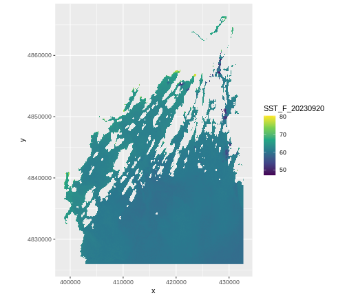
This is somewhat tedious. With the tidyterra package we
have another geom - geom_spatraster that deals with rasters
loaded by terra. Also, as land is NA in this data, it will
plot it quite nicely by default. We’ll also use
coord_sf()
R
ggplot() +
    geom_spatraster(data = b10_casco_2023,
                    aes(fill = SST_F_20230920)) +
    scale_fill_viridis_c()
OUTPUT
<SpatRaster> resampled to 500778 cells for plotting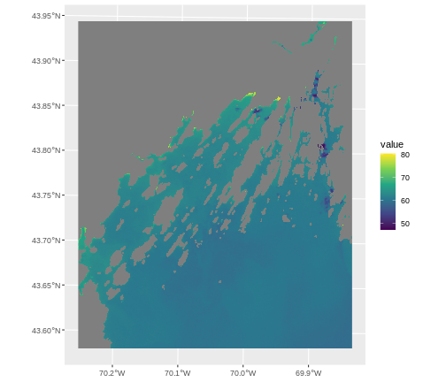
This looks great, and is now on the lat/long scale: CRS 4326. That’s
because spatial data is always plotted using the coord_sf()
coordinate system which defaults to 4326. If we want to show things in
another projection, or use the original one, we have to set a
datum argument.
R
ggplot() +
    geom_spatraster(data = b10_casco_2023,
                    aes(fill = SST_F_20230920)) +
    scale_fill_viridis_c() +
  coord_sf(datum = crs(b10_casco_2023, proj = TRUE))
OUTPUT
<SpatRaster> resampled to 500778 cells for plotting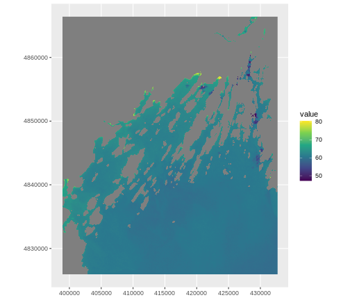
Plotting Tip
More information about the Viridis palette used above at R Viridis package documentation.
See ?plot for more arguments to customize the plot
R
plot(b10_casco_2023)
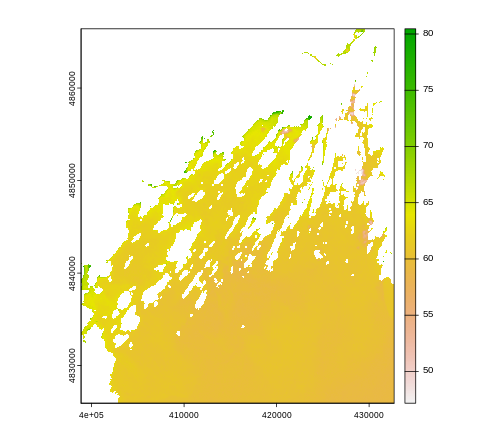
This map shows the sea surface temperature of our Casco Bay at one point in time in 2023. We can see that the maximum temperature is 80. While intuitively we know this is Farenheit (80C would be…. something), we don’t know for sure. We can look at the metadata of our object to see what the units are. Much of the metadata that we’re interested in is part of the CRS. We introduced the concept of a CRS in an earlier lesson.
Now we will see how features of the CRS appear in our data file and what meanings they have.
Understanding CRS in Proj4 Format
The CRS for our data is given to us by R in proj4
format. Let’s break down the pieces of proj4 string. The
string contains all of the individual CRS elements that R or another GIS
might need. Each element is specified with a + sign,
similar to how a .csv file is delimited or broken up by a
,. After each + we see the CRS element being
defined. For example projection (proj=) and datum
(datum=).
UTM Proj4 String
A projection string (like the one of b10_casco_2023)
specifies the UTM projection as follows:
+proj=utm +zone=19 +datum=WGS84 +units=m +no_defs
- proj=utm: the projection is UTM, UTM has several zones.
- zone=19: the zone is 19
- datum=WGS84: the datum is WGS84 (the datum refers to the 0,0 reference for the coordinate system used in the projection)
- units=m: the units for the coordinates are in meters
Note that the zone is unique to the UTM projection. Not all CRSs will have a zone. Image source: Chrismurf at English Wikipedia, via Wikimedia Commons (CC-BY).
Calculate Raster Min and Max Values
It is useful to know the minimum or maximum values of a raster dataset. In this case, given we are working with temperature data, these values represent the min/max sea surface temperature range in Casco Bay.
Raster statistics are often calculated and embedded in a GeoTIFF for us. We can view these values:
R
minmax(b10_casco_2023)
OUTPUT
    SST_F_20230920
min       47.09686
max       80.46152
R
min(values(b10_casco_2023), na.rm = TRUE)
OUTPUT
[1] 47.09686R
max(values(b10_casco_2023), na.rm = TRUE)
OUTPUT
[1] 80.46152We can see that the temperature at our site ranges from ~47F to ~80F.
Raster Bands
The Sea Surface Temperature object (b10_casco_2023) that
we’ve been working with is a single band raster. This means that there
is only one data set stored in the raster: SST at one time point.
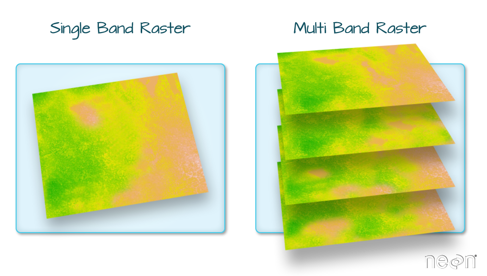
A raster dataset can contain one or more bands. We can use the
rast() function to import one single band from a single or
multi-band raster. We can view the number of bands in a raster using the
nlyr() function.
R
nlyr(b10_casco_2023)
OUTPUT
[1] 1However, raster data can also be multi-band, meaning that one raster
file contains data for more than one variable or time period for each
cell. By default the raster() function only imports the
first band in a raster regardless of whether it has one or more bands.
Jump to a later episode in this series for information on working with
multi-band rasters: Work with
Multi-band Rasters in R.
Bad Data Values in Rasters
Sometimes your rasters can have bad data values. These are different
from NoData Values, which get represented by NAs. Bad data
values are values that fall outside of the applicable range of a
dataset.
Examples of Bad Data Values:
- The normalized difference vegetation index (NDVI), which is a measure of greenness, has a valid range of -1 to 1. Any value outside of that range would be considered a “bad” or miscalculated value.
- Reflectance data in an image will often range from 0-1 or 0-10,000
depending upon how the data are scaled. Thus a value greater than 1 or
greater than 10,000 is likely caused by an error in either data
collection or processing.
- Coastal ocean data could be contaminated by measurements from land.
Find Bad Data Values
Sometimes a raster’s metadata will tell us the range of expected values for a raster. Values outside of this range are suspect and we need to consider that when we analyze the data. Sometimes, we need to use some common sense and scientific insight as we examine the data - just as we would for field data to identify questionable values.
Plotting data with appropriate highlighting can help reveal patterns in bad values and may suggest a solution. For example, let’s look at the range of our SST raster.
R
minmax(b10_casco_2023)
OUTPUT
    SST_F_20230920
min       47.09686
max       80.46152
47F seems reasonable, but 80? Maybe it is. But maybe it’s just land
values that bled over. Let’s assume 75F is the real maximum. To view
where we might have bad data, we can use classify() which
takes a matrix with three columns. The first is a low value. The second
is a high value. And the third is how we want that classified. Let’s say
we wanted to look at bad values in our SST dataset.
R
# reclassify raster to ok/not ok
range_matrix <- matrix(c(
  40,75, 1, #low, high, make a 1
  75, 90, 2
), ncol = 3, byrow = TRUE)

b10_highvals <- classify(b10_casco_2023,
                         rcl = range_matrix)

plot(b10_highvals)
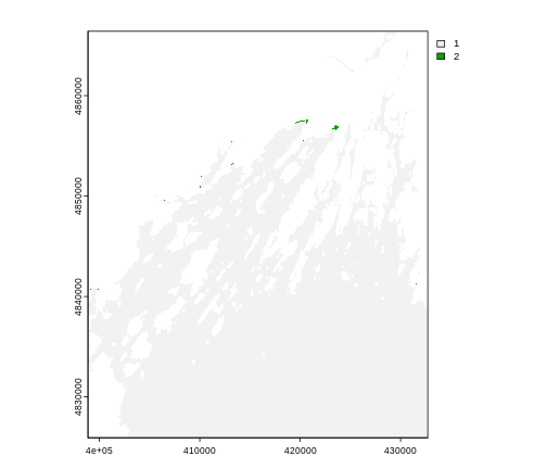
Yeah, it’s some spots at the tail-end of the coast that could indeed
by pixels contaminated by land. To fix that, we can set values outside
of our range to NA using clamp()
R
b10_casco_2023 <- clamp(b10_casco_2023,
                        lower = 40,
                        upper = 75)

minmax(b10_casco_2023)
OUTPUT
    SST_F_20230920
min       47.09686
max       75.00000
Create A Histogram of Raster Values
We can explore the distribution of values contained within our raster
using the geom_histogram() function which produces a
histogram. Histograms are often useful in identifying outliers and bad
data values in our raster data.
R
ggplot() +
    geom_histogram(data = b10_casco_2023_df,
                   mapping = aes(x = SST_F_20230920))
OUTPUT
`stat_bin()` using `bins = 30`. Pick better value with `binwidth`.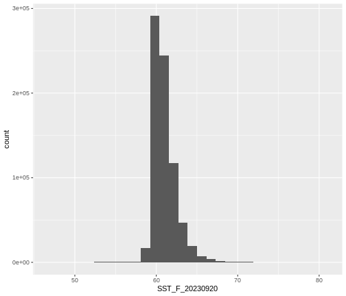
Notice that a warning message is thrown when R creates the histogram.
stat_bin() using bins = 30. Pick better
value with binwidth.
This warning is caused by a default setting in
geom_histogram enforcing that there are 30 bins for the
data. We can define the number of bins we want in the histogram by using
the bins value in the geom_histogram()
function.
R
ggplot() +
    geom_histogram(data = b10_casco_2023_df,
                   mapping = aes(x = SST_F_20230920),
                   bins = 100)
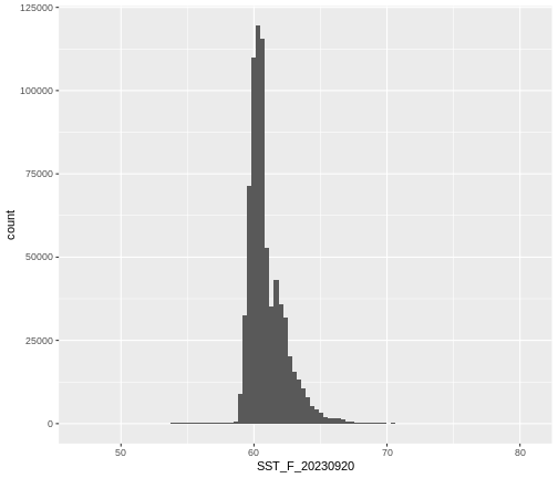
Note that the shape of this histogram looks similar to the previous one that was created using the default of 30 bins. The distribution of SST values looks reasonable. Although, we can see some very thin tails that we might want to inspect to see if they are real values or bad data.
Challenge: Explore Raster Metadata
Use describe() to determine the following about the
data/landsat_casco/b10_cropped/LC08_L2SP_011030_20130815_20200912_02_T1_ST_B10.TIF
file:
- Does this file have the same CRS as
b10_casco_2023_df? - What is the
NoData Value? - What is resolution of the raster data?
- How large would a 5x5 pixel area be on the Earth’s surface?
- Is the file a multi- or single-band raster?
R
describe("data/landsat_casco/b10_cropped/LC08_L2SP_011030_20130815_20200912_02_T1_ST_B10.TIF")
OUTPUT
 [1] "Driver: GTiff/GeoTIFF"
 [2] "Files: data/landsat_casco/b10_cropped/LC08_L2SP_011030_20130815_20200912_02_T1_ST_B10.TIF"
 [3] "Size is 1128, 1349"
 [4] "Coordinate System is:"
 [5] "PROJCRS[\"WGS 84 / UTM zone 19N\","
 [6] "    BASEGEOGCRS[\"WGS 84\","
 [7] "        DATUM[\"World Geodetic System 1984\","
 [8] "            ELLIPSOID[\"WGS 84\",6378137,298.257223563,"
 [9] "                LENGTHUNIT[\"metre\",1]]],"
[10] "        PRIMEM[\"Greenwich\",0,"
[11] "            ANGLEUNIT[\"degree\",0.0174532925199433]],"
[12] "        ID[\"EPSG\",4326]],"
[13] "    CONVERSION[\"UTM zone 19N\","
[14] "        METHOD[\"Transverse Mercator\","
[15] "            ID[\"EPSG\",9807]],"
[16] "        PARAMETER[\"Latitude of natural origin\",0,"
[17] "            ANGLEUNIT[\"degree\",0.0174532925199433],"
[18] "            ID[\"EPSG\",8801]],"
[19] "        PARAMETER[\"Longitude of natural origin\",-69,"
[20] "            ANGLEUNIT[\"degree\",0.0174532925199433],"
[21] "            ID[\"EPSG\",8802]],"
[22] "        PARAMETER[\"Scale factor at natural origin\",0.9996,"
[23] "            SCALEUNIT[\"unity\",1],"
[24] "            ID[\"EPSG\",8805]],"
[25] "        PARAMETER[\"False easting\",500000,"
[26] "            LENGTHUNIT[\"metre\",1],"
[27] "            ID[\"EPSG\",8806]],"
[28] "        PARAMETER[\"False northing\",0,"
[29] "            LENGTHUNIT[\"metre\",1],"
[30] "            ID[\"EPSG\",8807]]],"
[31] "    CS[Cartesian,2],"
[32] "        AXIS[\"(E)\",east,"
[33] "            ORDER[1],"
[34] "            LENGTHUNIT[\"metre\",1]],"
[35] "        AXIS[\"(N)\",north,"
[36] "            ORDER[2],"
[37] "            LENGTHUNIT[\"metre\",1]],"
[38] "    USAGE["
[39] "        SCOPE[\"Engineering survey, topographic mapping.\"],"
[40] "        AREA[\"Between 72°W and 66°W, northern hemisphere between equator and 84°N, onshore and offshore. Aruba. Bahamas. Brazil. Canada - New Brunswick (NB); Labrador; Nunavut; Nova Scotia (NS); Quebec. Colombia. Dominican Republic. Greenland. Netherlands Antilles. Puerto Rico. Turks and Caicos Islands. United States. Venezuela.\"],"
[41] "        BBOX[0,-72,84,-66]],"
[42] "    ID[\"EPSG\",32619]]"
[43] "Data axis to CRS axis mapping: 1,2"
[44] "Origin = (398865.000000000000000,4866405.000000000000000)"
[45] "Pixel Size = (30.000000000000000,-30.000000000000000)"
[46] "Metadata:"
[47] "  AREA_OR_POINT=Area"
[48] "Image Structure Metadata:"
[49] "  COMPRESSION=LZW"
[50] "  INTERLEAVE=BAND"
[51] "Corner Coordinates:"
[52] "Upper Left  (  398865.000, 4866405.000) ( 70d15'36.90\"W, 43d56'37.75\"N)"
[53] "Lower Left  (  398865.000, 4825935.000) ( 70d15' 9.45\"W, 43d34'46.27\"N)"
[54] "Upper Right (  432705.000, 4866405.000) ( 69d50'19.04\"W, 43d56'51.69\"N)"
[55] "Lower Right (  432705.000, 4825935.000) ( 69d50' 0.77\"W, 43d35' 0.04\"N)"
[56] "Center      (  415785.000, 4846170.000) ( 70d 2'46.52\"W, 43d45'49.65\"N)"
[57] "Band 1 Block=1128x1 Type=Float32, ColorInterp=Gray"
[58] "  Description = SST_F_20130815"
[59] "  Min=51.010 Max=89.659 "
[60] "  Minimum=51.010, Maximum=89.659, Mean=-9999.000, StdDev=-9999.000"
[61] "  NoData Value=nan"
[62] "  Metadata:"
[63] "    STATISTICS_MAXIMUM=89.659408569336"
[64] "    STATISTICS_MEAN=-9999"
[65] "    STATISTICS_MINIMUM=51.00980758667"
[66] " STATISTICS_STDDEV=-9999" - If this file has the same CRS as DSM_HARV? Yes: UTM Zone 19, WGS84, meters.
- What format
NoData Valuestake? 0 - The resolution of the raster data? 1x1
- How large a 5x5 pixel area would be? 5mx5m How? We are given resolution of 1x1 and units in meters, therefore resolution of 5x5 means 5x5m.
- Is the file a multi- or single-band raster? Single.
Content from Plot Raster Data
Last updated on 2024-03-12 | Edit this page
Estimated time: 70 minutes
WARNING
Warning in
download.file("https://www.naturalearthdata.com/http//www.naturalearthdata.com/download/110m/physical/ne_110m_graticules_all.zip",
: cannot open URL
'https://www.naturalearthdata.com/http//www.naturalearthdata.com/download/110m/physical/ne_110m_graticules_all.zip':
HTTP status was '500 Internal Server Error'
ERROR
Error in download.file("https://www.naturalearthdata.com/http//www.naturalearthdata.com/download/110m/physical/ne_110m_graticules_all.zip", : cannot open URL 'https://www.naturalearthdata.com/http//www.naturalearthdata.com/download/110m/physical/ne_110m_graticules_all.zip'Overview
Questions
- How can I create categorized or customized maps of raster data?
- How can I customize the color scheme of a raster image?
- How can I make my visualizations interactive?
Objectives
- Build customized plots for a single band raster using the
ggplot2package. - Make interactive maps with leaflet
First, let’s load some libraries. You should have them loaded from the previous less, but in case you don’t -
R
library(terra)
library(tidyterra)
library(ggplot2)
library(dplyr)
We are also going to load one new library.
R
library(leaflet)
To remind you, this is the data we will be using -
R
# Learners will have this data loaded from earlier episode
# DSM data for Harvard Forest
b10_casco_2023 <-
  rast("data/landsat_casco/b10_cropped/LC09_L2SP_011030_20230920_20230922_02_T1_ST_B10.TIF") |>
  clamp(lower = 50,
        upper = 75)

b10_casco_2023_df <- as.data.frame(b10_casco_2023, xy = TRUE)
Things You’ll Need To Complete This Episode
See the lesson homepage for detailed information about the software, data, and other prerequisites you will need to work through the examples in this episode.
Plot Raster Data in R
This episode covers how to plot a raster in R using the
ggplot2 package with customized coloring schemes. We will
then make interactive maps with leaflet.
We will continue working with the Landsat SST data from Casco Bay.
Plotting Data Using Breaks
In the previous episode, we viewed our data using a continuous color
ramp. For clarity and visibility of the plot - or if there are classes
you are interested in - we may prefer to view the data “symbolized” or
colored according to ranges of values. This is comparable to a
“classified” map. To do this, we need to tell ggplot how
many groups to break our data into, and where those breaks should be. To
make these decisions, it is useful to first explore the distribution of
the data using a bar plot. To begin with, we will use
dplyr’s mutate() function combined with
cut() to split the data into 4 bins.
R
b10_casco_2023_df <- b10_casco_2023_df %>%
                mutate(fct_sst = cut(SST_F_20230920, breaks = 4))

ggplot() +
    geom_bar(data = b10_casco_2023_df, aes(fct_sst))
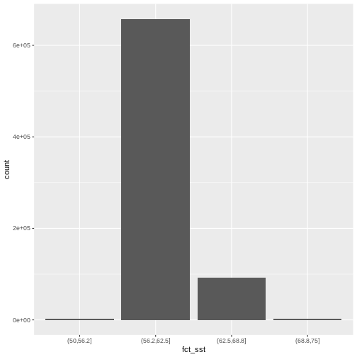
If we want to know the cutoff values for the groups, we can ask for
the unique values of fct_sst:
R
unique(b10_casco_2023_df$fct_sst)
OUTPUT
[1] (62.5,68.8] (68.8,75]   (56.2,62.5] (50,56.2]
Levels: (50,56.2] (56.2,62.5] (62.5,68.8] (68.8,75]
And we can get the count of values in each group using
dplyr’s group_by() and count()
functions:
R
b10_casco_2023_df %>%
        group_by(fct_sst) %>%
        count()
OUTPUT
# A tibble: 4 × 2
# Groups:   fct_sst [4]
  fct_sst          n
  <fct>        <int>
1 (50,56.2]     2370
2 (56.2,62.5] 657710
3 (62.5,68.8]  92571
4 (68.8,75]     2461
We might prefer to customize the cutoff values for these groups. Lets
round the cutoff values so that we have groups for the ranges of 50 –
55F, 55 – 60F, 65 - 70F and 70-75F. To implement this we will give
mutate() a numeric vector of break points instead of the
number of breaks we want.
R
custom_bins <- c(50, 55, 60, 65, 70, 75)

b10_casco_2023_df <- b10_casco_2023_df %>%
  mutate(fct_sst_2 = cut(SST_F_20230920, breaks = custom_bins))

unique(b10_casco_2023_df$fct_sst_2)
OUTPUT
[1] (65,70] (70,75] (60,65] (55,60] (50,55] <NA>
Levels: (50,55] (55,60] (60,65] (65,70] (70,75]
cut() is a powerful function, and there are a series of
related ones that are quite useful.
| function | what it does |
|---|---|
| cut | makes groups based on pre-defined breakpoints |
| cut_interval | makes n groups with equal range |
| cut_width | makes groups with a given width |
| cut_number | makes n groups with an equal number of observations |
Try them out with b10_casco_2023_df$SST_F_20230920 to
see how they differ.
And now we can plot our bar plot again, using the new groups:
R
ggplot() +
  geom_bar(data = b10_casco_2023_df,
           mapping = aes(fct_sst_2))
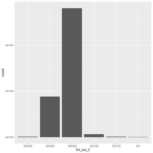
And we can get the count of values in each group in the same way we did before:
R
b10_casco_2023_df %>%
  group_by(fct_sst_2) %>%
  count()
OUTPUT
# A tibble: 6 × 2
# Groups:   fct_sst_2 [6]
  fct_sst_2      n
  <fct>      <int>
1 (50,55]     1483
2 (55,60]   176310
3 (60,65]   562050
4 (65,70]    13284
5 (70,75]     1715
6 <NA>         270
We can use those groups to plot our raster data, with each group
being a different color. We could do this with our data frame, or, we
can use the scale_color_binned() color scale. This is a
feature of ggplot2 that lets you create bins on the fly and
plot them. We can specify our custom breaks with the breaks
argument.
R
ggplot() +
  geom_spatraster(data = b10_casco_2023) +
  scale_fill_binned(breaks = custom_bins)
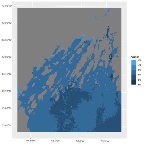
A lot of color scales have binned versions. We could have done the
above with scale_fill_viridis_b(). Or we could place with
scale_fill_fermenter() which comes from Color Brewer.
R
ggplot() +
  geom_spatraster(data = b10_casco_2023) +
  scale_fill_fermenter(breaks = custom_bins,
                       palette = "Accent")
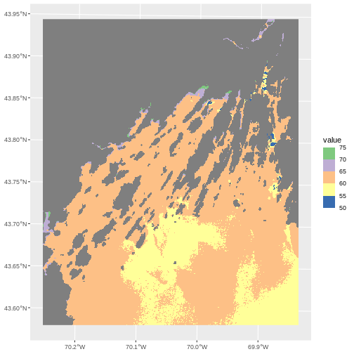
Note the choices of palette. ColorBrewer supplies quite a few to try!
R
RColorBrewer::display.brewer.all()
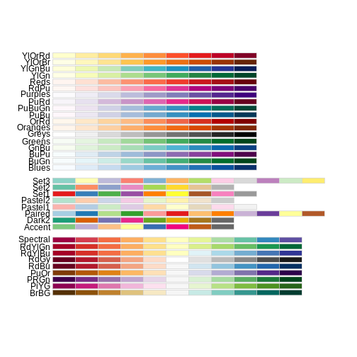
This is just the tip of the iceberg when looking for color palettes
for R, and it’s a topic well worth searching out when you want to
customize your own plots to the nth degree. You can even make your own
custom palette with scale_fill_stepsn().
R
my_pal <- c("red", "blue", "purple", "orange", "yellow")

ggplot() +
  geom_spatraster(data = b10_casco_2023) +
  scale_fill_stepsn(breaks = custom_bins,,
                    colors = my_pal)
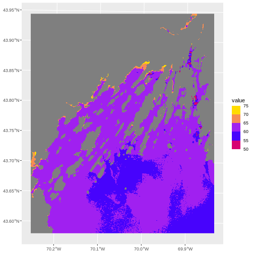
One advantage to this is that you can then use the same breaks and
color palette across multiple plots for consistency, rather than having
ggplot2 choose the breaks and palette stretching for you.
There are also many wonderful palette packages, like wesanderson or beyonce.
More Plot Formatting
All labels in a plot can be controlled by the labs()
function. So, if we wanted to give the fill name “SST (F)”, label the X
and Y axis, and give this plot a title of “SST on Sept 9, 2023” we can
do so easily.
R
ggplot() +
  geom_spatraster(data = b10_casco_2023) +
  scale_fill_stepsn(breaks = custom_bins,,
                    colors = my_pal) +
  labs(title = "SST on Sept 9, 2023",
       x = "Longitude", y = "Latitude",
       fill = "SST (F)")
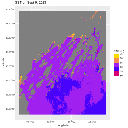
We can also retheme the entire plot - changing the background, axis options, and more. If you really want to get deeply into themes, there are many wonderful packages out there like ggthemes, tvthemes, hrbrthemes, ggsci, and so many more.
Within ggplot itself, chekc out the different theme_*()
functions, such as theme_void(). We can use the
base_size argument to specify a base font size as well.
R
ggplot() +
  geom_spatraster(data = b10_casco_2023) +
  scale_fill_stepsn(breaks = custom_bins,,
                    colors = my_pal) +
  labs(title = "SST on Sept 9, 2023",
       x = "Longitude", y = "Latitude",
       fill = "SST (F)") +
  theme_void(base_size = 12)
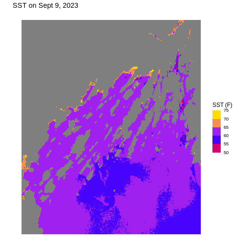
You can also make your own custom theme or theme modifications with
the theme() function. Dig into the ?theme
helpfile to learn more and see examples.
Challenge: Plot Using Custom Breaks
Create a plot of the Casco Bay SST in August 2013 that has:
- Three classified ranges of values (break points) that are evenly divided among the range of pixel values. Any palette you’d like!
- Axis labels.
- A plot title.
- A unique theme.
The file is
data/landsat_casco/b10_cropped/LC08_L2SP_011030_20130815_20200912_02_T1_ST_B10.TIF
to remind you.
R
b10_casco_2013 <- rast("data/landsat_casco/b10_cropped/LC08_L2SP_011030_20130815_20200912_02_T1_ST_B10.TIF")

# find intervals
cut_interval(values(b10_casco_2013), n = 3) |> levels()

# round those intervals into breaks
new_breaks <- c(50, 65, 75, 85)

# plot with these new breaks using Set2 as the palette

ggplot() +
  geom_spatraster(data = b10_casco_2013) +
  scale_fill_fermenter(breaks = new_breaks,
                    palette = "Set2") +
  labs(title = "SST on Aug 15, 2023",
       x = "Longitude", y = "Latitude",
       fill = "SST (F)") +
  ggthemes::theme_few()
Interactive Maps
These static maps are beautiful, but, they can be difficult if you notice features occurring at small scales you want to investigate. They’re also wonderful objects to build for web applications and the like, as they allow users a degree of interactivity.
For a basic level of interactivity - just to explore -
terra includes a function called plet() which
lets us look at our raster interactively.
R
plet(b10_casco_2023)
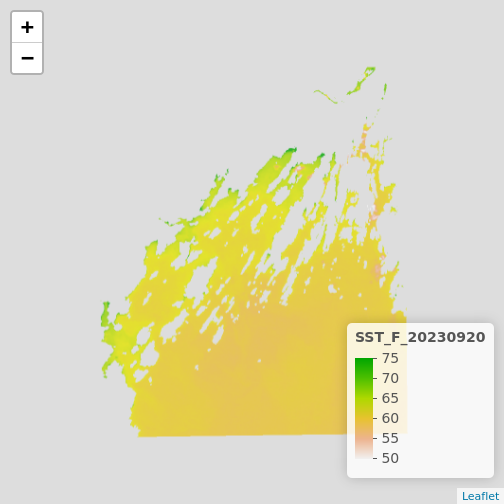
This is great, and we can even put some reference behind it with the
tiles argument.
R
plet(b10_casco_2023, tile = "Esri.WorldImagery")
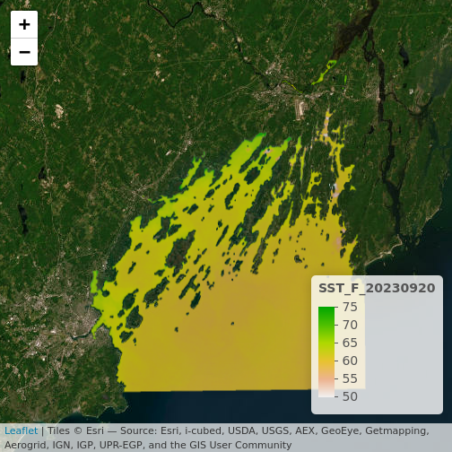
What do you learn from this?
R
plet(b10_casco_2023, tile = "Street")
Data Tips
If you want to make sure things can be seen behind the raster, try
fiddling with the alpha values. It’s set to 0.8 by default
The alpha value determines how transparent the colors will be (0 being
transparent, 1 being opaque).
There are other options for plet that could be well
worth an exploration as you use it to try and understand what is
happening in your raster imagery.
The above is well and good for exploration, but for presentation you
might something more customized. Did you notice in the lowe right-hand
corner the word “leaflet”? This is the name of a Javascript library that
powers a lot of interactive maps you see on the internet.
plet() actually calls an R library leaflet
that then interacts with the Javascript library to make these maps. You
can learn a lot more about leaflet for R from here.
The leaflet library works in some very similar and some
very different ways from ggplot2. It’s useful to know as it
allows us to customize the presentation of our maps for a public
audience. It works by building a map up in a sequence of layers, like
ggplot2, except that it uses the pipe to add each new
element. For example, to generate the above map, we’d have to first
initialize a leaflet() map, then addTiles(),
and finally addRasterImage().
R
library(leaflet)

leaflet() |>
  addTiles() |>
  addRasterImage(b10_casco_2023)
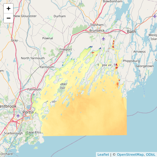
Note that the color palette is different as is the background map
from plet(). This is all customizable!
addTiles() takes an argument urlTemplate
which looks a bit odd, but, you can get the arguments for different
tilesets from this
site. Or use addProviderTiles() to just specify a
provider and map.
R
leaflet() |>
  addProviderTiles("Esri.WorldImagery") |>
  addRasterImage(b10_casco_2023, opacity = 0.8)
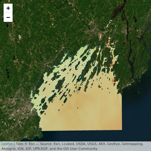
For colors, we can specify a color mapping - from our raster to a
palette. There are four functions for this. colorNumeric()
is for continuous values. colorBin() does what we’ve been
doing with scale_fill_binned(). We can use discrete values
with colorFactor() or if we want to use quantiles (e.g., to
highlight 95th percentiles and extremes beyond them), we can use
colorQuantile(). Each takes a palette, which we can either
specify as a vector of colors or a name of a ColorBrewer or Viridis
palette. It also takes a domain, the values the palette will be mapped
to.
What’s great about defining a palette here is that we can then use it
for addLegend() or for other maps to have equivalent
scales. Here’s an example using the RdYlBu palette. Don’t
forget to set na.color = "transparent" if you don’t want to
see it.
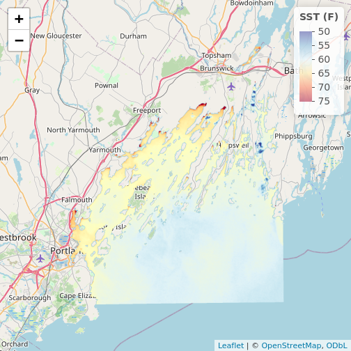
R
# note, using reverse = TRUE here as otherwise warm = blue
my_pal <- colorNumeric(palette = "RdYlBu",
                    domain = values(b10_casco_2023),
                    na.color = "transparent",
                    reverse = TRUE)

leaflet() |>
  addTiles() |>
  addRasterImage(b10_casco_2023,
                 colors = my_pal) |>
  addLegend(pal = my_pal,
            values = values(b10_casco_2023),
            title = "SST (F)")
R
# Let's do bins!
new_pal <- colorBin(palette = "plasma",
                    domain = values(b10_casco_2013),
                    na.color = "transparent")

leaflet() |>
  addProviderTiles("Esri.WorldTerrain") |>
  addProviderTiles("Thunderforest.SpinalMap") |>
  addProviderTiles("Esri.WorldImagery") |>
  addRasterImage(b10_casco_2013,
                 colors = new_pal,
                 opacity = 0.7) |>
  addLegend(pal = new_pal,
            values = values(b10_casco_2013),
            title = "SST (F)") |>
  addScaleBar("bottomleft") |>
  addLayersControl(position = "bottomright",
                   baseGroups = c("World Terrain",
                                  "This Is Spinal Map!",
                                  "World Imagery"))
Key Points
- Continuous data ranges can be grouped into categories using
mutate()andcut()or with a binned color scale inggplot2. - Use built-in color palettes with
scale_fill_viridis_borscale_fill_fermenter()or set your preferred color scheme manually. - Interactive plotting with
plet()and theleafletlibrary can lead to even better insights as you zoom in and out.
Content from Open and Plot Vector Layers
Last updated on 2024-03-12 | Edit this page
Estimated time: 30 minutes
WARNING
Warning in
download.file("https://www.naturalearthdata.com/http//www.naturalearthdata.com/download/110m/physical/ne_110m_graticules_all.zip",
: cannot open URL
'https://www.naturalearthdata.com/http//www.naturalearthdata.com/download/110m/physical/ne_110m_graticules_all.zip':
HTTP status was '500 Internal Server Error'
ERROR
Error in download.file("https://www.naturalearthdata.com/http//www.naturalearthdata.com/download/110m/physical/ne_110m_graticules_all.zip", : cannot open URL 'https://www.naturalearthdata.com/http//www.naturalearthdata.com/download/110m/physical/ne_110m_graticules_all.zip'Overview
Questions
- How can I distinguish between and visualize point, line and polygon vector data?
Objectives
- Know the difference between point, line, and polygon vector elements.
- Load point, line, and polygon vector layers into R.
- Access the attributes of a spatial object in R.
First, some libraries you might not have loaded at the moment.
R
library(terra)
library(ggplot2)
library(dplyr)
library(sf)
Things You’ll Need To Complete This Episode
See the lesson homepage for detailed information about the software, data, and other prerequisites you will need to work through the examples in this episode.
Starting with this episode, we will be moving from working with
raster data to working with vector data. In this episode, we will open
and plot point, line and polygon vector data loaded from ESRI’s
shapefile format into R. These data refer to data from the
Maine GeoLibrary
Data Catalogue on seagrass beds, public roads, and boat launches. In
later episodes, we will learn how to work with raster and vector data
together and combine them into a single plot.
Import Vector Data
We will use the sf package to work with vector data in
R. We will also use the terra package, which has been
loaded in previous episodes, so we can explore raster and vector spatial
metadata using similar commands. Make sure you have the sf
library loaded.
R
library(sf)
The vector layers that we will import from ESRI’s
shapefile format are:
- A polygon vector layer representing our field site boundary,
- A line vector layer representing the public roads of Maine, and
- A point vector layer representing the location of the boat launches around Maine.
The first vector layer that we will open contains the boundary of our
study area (or our Area Of Interest or AOI, hence the name
aoiBoundary). To import a vector layer from an ESRI
shapefile we use the sf function
st_read(). st_read() requires the file path to
the ESRI shapefile.
Let’s import our AOI:
R
aoi_boundary_casco <- st_read(
  "data/maine_gov_maps/casco_aoi/casco_bay_aoi.shp")
OUTPUT
Reading layer `casco_bay_aoi' from data source
  `/home/runner/work/r-raster-vector-geospatial/r-raster-vector-geospatial/site/built/data/maine_gov_maps/casco_aoi/casco_bay_aoi.shp'
  using driver `ESRI Shapefile'
Simple feature collection with 1 feature and 1 field
Geometry type: POLYGON
Dimension:     XY
Bounding box:  xmin: -70.2528 ymin: 43.5834 xmax: -69.8387 ymax: 43.9439
Geodetic CRS:  WGS 84
Vector Layer Metadata & Attributes
When we import the casco_bay_aoi.shp vector layer from
an ESRI shapefile into R (as our
aoi_boundary_casco object), the st_read()
function automatically stores information about the data. We are
particularly interested in the geospatial metadata, describing the
format, CRS, extent, and other components of the vector data, and the
attributes which describe properties associated with each individual
vector object.
Data Tip
The Explore and Plot by Vector Layer Attributes episode provides more information on both metadata and attributes and using attributes to subset and plot data.
Spatial Metadata
Key metadata for all vector layers includes:
- Object Type: the class of the imported object.
- Coordinate Reference System (CRS): the projection of the data.
- Extent: the spatial extent (i.e. geographic area that the vector layer covers) of the data. Note that the spatial extent for a vector layer represents the combined extent for all individual objects in the vector layer.
We can view metadata of a vector layer using the
st_geometry_type(), st_crs() and
st_bbox() functions. First, let’s view the geometry type
for our AOI vector layer:
R
st_geometry_type(aoi_boundary_casco)
OUTPUT
[1] POLYGON
18 Levels: GEOMETRY POINT LINESTRING POLYGON MULTIPOINT ... TRIANGLE
Our aoi_boundary_casco is a polygon spatial object. The
18 levels shown below our output list the possible categories of the
geometry type. Now let’s check what CRS this file data is in:
R
st_crs(aoi_boundary_casco)
OUTPUT
Coordinate Reference System:
  User input: WGS 84
  wkt:
GEOGCRS["WGS 84",
    DATUM["World Geodetic System 1984",
        ELLIPSOID["WGS 84",6378137,298.257223563,
            LENGTHUNIT["metre",1]]],
    PRIMEM["Greenwich",0,
        ANGLEUNIT["degree",0.0174532925199433]],
    CS[ellipsoidal,2],
        AXIS["latitude",north,
            ORDER[1],
            ANGLEUNIT["degree",0.0174532925199433]],
        AXIS["longitude",east,
            ORDER[2],
            ANGLEUNIT["degree",0.0174532925199433]],
    ID["EPSG",4326]]
Our data in the CRS WGS 84 (it is EPSG code 4326).
The CRS is critical to interpreting the spatial object’s extent values
as it specifies units. To find the extent of our AOI, we can use the
st_bbox() function:
R
st_bbox(aoi_boundary_casco)
OUTPUT
    xmin     ymin     xmax     ymax
-70.2528  43.5834 -69.8387  43.9439
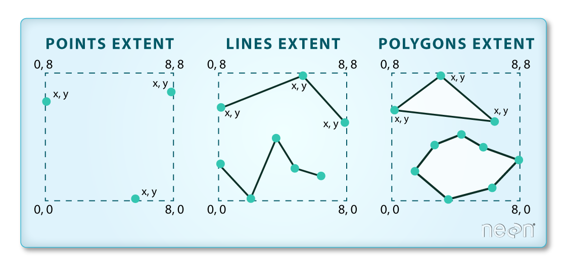
The spatial extent of a vector layer or R spatial object represents the geographic “edge” or location that is the furthest north, south east and west. Thus it represents the overall geographic coverage of the spatial object. Image Source: National Ecological Observatory Network (NEON).
Lastly, we can view all of the metadata and attributes for this R spatial object by printing it to the screen:
R
aoi_boundary_casco
OUTPUT
Simple feature collection with 1 feature and 1 field
Geometry type: POLYGON
Dimension:     XY
Bounding box:  xmin: -70.2528 ymin: 43.5834 xmax: -69.8387 ymax: 43.9439
Geodetic CRS:  WGS 84
  FID                       geometry
1   0 POLYGON ((-70.2528 43.5834,...
Spatial Data Attributes
We introduced the idea of spatial data attributes in an earlier lesson. Now we will explore how to use spatial data attributes stored in our data to plot different features.
Plot a vector layer
Next, let’s visualize the data in our sf object using
the ggplot package. Unlike with raster data, we do not need
to convert vector data to a dataframe before plotting with
ggplot.
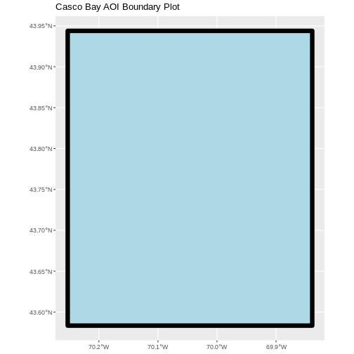
We’re going to customize our boundary plot by setting the size,
color, and fill for our plot. When plotting sf objects with
ggplot2, you need to use the coord_sf()
coordinate system.
R
ggplot() +
  geom_sf(data = aoi_boundary_casco, linewidth = 3,
          color = "black", fill = "lightblue") +
  ggtitle("Casco Bay AOI Boundary Plot") +
  coord_sf()
Challenge: Import Line and Point Vector Layers
Using the steps above, import the MaineDOT_Public_Roads and
Maine_Boat_Launches_GeoLibrary vector layers into R. Call the
MaineDOT_Public_Roads object roads_maine and the
Maine_Boat_Launches_GeoLibrary boatlaunches_maine.
Answer the following questions:
What type of R spatial object is created when you import each layer?
What is the CRS and extent for each object?
Do the files contain points, lines, or polygons?
How many spatial objects are in each file?
First we import the data:
R
roads_maine <- st_read("data/maine_gov_maps/MaineDOT_Public_Roads/MaineDOT_Public_Roads.shp")
OUTPUT
Reading layer `MaineDOT_Public_Roads' from data source
  `/home/runner/work/r-raster-vector-geospatial/r-raster-vector-geospatial/site/built/data/maine_gov_maps/MaineDOT_Public_Roads/MaineDOT_Public_Roads.shp'
  using driver `ESRI Shapefile'
Simple feature collection with 100669 features and 30 fields
Geometry type: LINESTRING
Dimension:     XY
Bounding box:  xmin: -71.04662 ymin: 43.06728 xmax: -66.95202 ymax: 47.35999
Geodetic CRS:  WGS 84
R
boatlaunches_maine <- st_read("data/maine_gov_maps/Maine_Boat_Launches_GeoLibrary/Maine_Boat_Launches_GeoLibrary.shp")
OUTPUT
Reading layer `Maine_Boat_Launches_GeoLibrary' from data source
  `/home/runner/work/r-raster-vector-geospatial/r-raster-vector-geospatial/site/built/data/maine_gov_maps/Maine_Boat_Launches_GeoLibrary/Maine_Boat_Launches_GeoLibrary.shp'
  using driver `ESRI Shapefile'
Simple feature collection with 578 features and 20 fields
Geometry type: POINT
Dimension:     XY
Bounding box:  xmin: -70.9817 ymin: 43.0859 xmax: -66.9838 ymax: 47.35484
Geodetic CRS:  WGS 84
Then we check its class:
R
class(roads_maine)
OUTPUT
[1] "sf" "data.frame"R
class(boatlaunches_maine)
OUTPUT
[1] "sf" "data.frame"We also check the CRS and extent of each object:
R
st_crs(roads_maine)
OUTPUT
Coordinate Reference System:
  User input: WGS 84
  wkt:
GEOGCRS["WGS 84",
    DATUM["World Geodetic System 1984",
        ELLIPSOID["WGS 84",6378137,298.257223563,
            LENGTHUNIT["metre",1]]],
    PRIMEM["Greenwich",0,
        ANGLEUNIT["degree",0.0174532925199433]],
    CS[ellipsoidal,2],
        AXIS["latitude",north,
            ORDER[1],
            ANGLEUNIT["degree",0.0174532925199433]],
        AXIS["longitude",east,
            ORDER[2],
            ANGLEUNIT["degree",0.0174532925199433]],
    ID["EPSG",4326]]
R
st_bbox(roads_maine)
OUTPUT
     xmin      ymin      xmax      ymax
-71.04662  43.06728 -66.95202  47.35999
R
st_crs(boatlaunches_maine)
OUTPUT
Coordinate Reference System:
  User input: WGS 84
  wkt:
GEOGCRS["WGS 84",
    DATUM["World Geodetic System 1984",
        ELLIPSOID["WGS 84",6378137,298.257223563,
            LENGTHUNIT["metre",1]]],
    PRIMEM["Greenwich",0,
        ANGLEUNIT["degree",0.0174532925199433]],
    CS[ellipsoidal,2],
        AXIS["latitude",north,
            ORDER[1],
            ANGLEUNIT["degree",0.0174532925199433]],
        AXIS["longitude",east,
            ORDER[2],
            ANGLEUNIT["degree",0.0174532925199433]],
    ID["EPSG",4326]]
R
st_bbox(boatlaunches_maine)
OUTPUT
     xmin      ymin      xmax      ymax
-70.98170  43.08590 -66.98380  47.35484
To see the number of objects in each file, we can look at the output
from when we read these objects into R. roads_maine
contains 100669 features (all lines) and boatlaunches_maine
contains 578 points.
Content from Explore and Plot by Vector Layer Attributes
Last updated on 2024-03-12 | Edit this page
Estimated time: 60 minutes
WARNING
Warning in
download.file("https://www.naturalearthdata.com/http//www.naturalearthdata.com/download/110m/physical/ne_110m_graticules_all.zip",
: cannot open URL
'https://www.naturalearthdata.com/http//www.naturalearthdata.com/download/110m/physical/ne_110m_graticules_all.zip':
HTTP status was '500 Internal Server Error'
ERROR
Error in download.file("https://www.naturalearthdata.com/http//www.naturalearthdata.com/download/110m/physical/ne_110m_graticules_all.zip", : cannot open URL 'https://www.naturalearthdata.com/http//www.naturalearthdata.com/download/110m/physical/ne_110m_graticules_all.zip'Overview
Questions
- How can I compute on the attributes of a spatial object?
Objectives
- Query attributes of a spatial object.
- Subset spatial objects using specific attribute values.
- Plot a vector feature, colored by unique attribute values.
Things You’ll Need To Complete This Episode
See the lesson homepage for detailed information about the software, data, and other prerequisites you will need to work through the examples in this episode.
This episode continues our discussion of vector layer attributes and covers how to work with vector layer attributes in R. It covers how to identify and query layer attributes, as well as how to subset features by specific attribute values. Finally, we will learn how to plot a feature according to a set of attribute values. We will do this looking at data regarding Seagrass beds in Casco Bay from 2022 provided by the Maine DEP. For full metadata, see here.
Load the Data
We will continue using the sf and ggplot2
packages in this episode. Make sure that you have these packages
loaded.
R
library(ggplot2)
library(dplyr)
library(sf)
We will continue to work with the ESRI shapefiles
(vector layers). Let’s start looking at seagrass beds around Casco Bay
from 2022.
R
# seagrass in 2022
seagrass_casco_2022 <- st_read(
  "data/maine_gov_seagrass/MaineDEP_Casco_Bay_Seagrass_2022/MaineDEP_Casco_Bay_Seagrass_2022.shp")
Query Vector Feature Metadata
As we discussed in the Open and Plot Vector Layers in R episode, we can view metadata associated with an R object using:
-
st_geometry_type()- The type of vector data stored in the object. -
nrow()- The number of features in the object -
st_bbox()- The spatial extent (geographic area covered by) of the object. -
st_crs()- The CRS (spatial projection) of the data.
We started to explore our seagrass_casco_2022 object To
see a summary of all of the metadata associated with our
seagrass_casco_2022 object, we can view the object with
View(seagrass_casco_2022) or print a summary of the object
itself to the console.
R
seagrass_casco_2022
OUTPUT
Simple feature collection with 622 features and 15 fields
Geometry type: POLYGON
Dimension:     XY
Bounding box:  xmin: -70.24464 ymin: 43.57213 xmax: -69.84399 ymax: 43.93221
Geodetic CRS:  WGS 84
First 10 features:
   OBJECTID Id Name       Acres   Hectares Orth_Cover Cover_Pct Field_Ver
1         1  1   01  0.04456005 0.01803281          1      0-10         Y
2         2  4   02  0.06076669 0.02459141          3     40-70         Y
3         3  6   03  2.56218247 1.03687846          3     40-70         Y
4         4  8   05  0.71816162 0.29062970          3     40-70         Y
5         5  9   06  0.01815022 0.00734513          3     40-70         Y
6         6 10   07  0.33051475 0.13375458          3     40-70         Y
7         7 11   08  0.08088664 0.03273366          1      0-10         Y
8         8 13   09  0.66689055 0.26988103          1      0-10         Y
9         9 14   10  0.03080650 0.01246695          3     40-70         Y
10       10 15   11 12.54074080 5.07505774          4    70-100         Y
   Video_YN                          Video Comment        Species
1         Y                            A03    <NA> Zostera marina
2         Y                            A04    <NA> Zostera marina
3         Y                            A05    <NA> Zostera marina
4         Y                            A07    <NA> Zostera marina
5         Y                            A08    <NA> Zostera marina
6         Y                            A09    <NA> Zostera marina
7         Y                            A10    <NA> Zostera marina
8         Y                            A11    <NA> Zostera marina
9         Y                            A12    <NA> Zostera marina
10        Y A14, A15, A16, A17, SP07, SP08    <NA> Zostera marina
                                 GlobalID  ShapeSTAre ShapeSTLen
1  {7CAB9D54-4BF9-4B91-94D6-4F0EA4AD53C1}   180.32842  102.57257
2  {D5396F39-D508-45CB-BFE0-13A506D4E94C}   245.91500   84.35420
3  {3C1ED4DC-6580-4CAC-9499-32D445019068} 10368.78375  719.04025
4  {6C1395B8-F532-46C6-AFBA-23B14C2F2E02}  2906.29561  315.88722
5  {EDEDAFA1-8605-4FAC-910F-E6E864F51209}    73.45108   34.00204
6  {820DE3B5-BA6E-4415-A110-95F9F94A4F1C}  1337.54527  165.98655
7  {E4E2A155-7B1C-46C3-94B5-6D0E58B1FEBB}   327.33664  112.52478
8  {C7FEF8AC-9BA7-429C-A45B-270E836FBBA1}  2698.81099  295.01388
9  {356C58A4-DB72-445F-83DA-1035C8EAE917}   124.66947   43.47523
10 {C797140E-F9CB-4EA0-9D7C-FBEA50FE9EB2} 50750.58217 1949.02908
                         geometry
1  POLYGON ((-70.20081 43.5722...
2  POLYGON ((-70.20228 43.5869...
3  POLYGON ((-70.20858 43.5909...
4  POLYGON ((-70.21488 43.5924...
5  POLYGON ((-70.21499 43.5931...
6  POLYGON ((-70.21582 43.5963...
7  POLYGON ((-70.21618 43.5964...
8  POLYGON ((-70.21641 43.5971...
9  POLYGON ((-70.21498 43.6063...
10 POLYGON ((-70.22445 43.6425...
We can use the ncol function to count the number of
attributes associated with a spatial object too. Note that the geometry
is just another column and counts towards the total.
R
ncol(seagrass_casco_2022)
OUTPUT
[1] 16We can view the individual name of each attribute using the
names() function in R:
R
names(seagrass_casco_2022)
OUTPUT
 [1] "OBJECTID"   "Id"         "Name"       "Acres"      "Hectares"
 [6] "Orth_Cover" "Cover_Pct"  "Field_Ver"  "Video_YN"   "Video"
[11] "Comment"    "Species"    "GlobalID"   "ShapeSTAre" "ShapeSTLen"
[16] "geometry"
We could also view just the first 6 rows of attribute values using
the head() function to get a preview of the data:
R
head(seagrass_casco_2022)
OUTPUT
Simple feature collection with 6 features and 15 fields
Geometry type: POLYGON
Dimension:     XY
Bounding box:  xmin: -70.21582 ymin: 43.57213 xmax: -70.20057 ymax: 43.59667
Geodetic CRS:  WGS 84
  OBJECTID Id Name      Acres   Hectares Orth_Cover Cover_Pct Field_Ver
1        1  1   01 0.04456005 0.01803281          1      0-10         Y
2        2  4   02 0.06076669 0.02459141          3     40-70         Y
3        3  6   03 2.56218247 1.03687846          3     40-70         Y
4        4  8   05 0.71816162 0.29062970          3     40-70         Y
5        5  9   06 0.01815022 0.00734513          3     40-70         Y
6        6 10   07 0.33051475 0.13375458          3     40-70         Y
  Video_YN Video Comment        Species                               GlobalID
1        Y   A03    <NA> Zostera marina {7CAB9D54-4BF9-4B91-94D6-4F0EA4AD53C1}
2        Y   A04    <NA> Zostera marina {D5396F39-D508-45CB-BFE0-13A506D4E94C}
3        Y   A05    <NA> Zostera marina {3C1ED4DC-6580-4CAC-9499-32D445019068}
4        Y   A07    <NA> Zostera marina {6C1395B8-F532-46C6-AFBA-23B14C2F2E02}
5        Y   A08    <NA> Zostera marina {EDEDAFA1-8605-4FAC-910F-E6E864F51209}
6        Y   A09    <NA> Zostera marina {820DE3B5-BA6E-4415-A110-95F9F94A4F1C}
   ShapeSTAre ShapeSTLen                       geometry
1   180.32842  102.57257 POLYGON ((-70.20081 43.5722...
2   245.91500   84.35420 POLYGON ((-70.20228 43.5869...
3 10368.78375  719.04025 POLYGON ((-70.20858 43.5909...
4  2906.29561  315.88722 POLYGON ((-70.21488 43.5924...
5    73.45108   34.00204 POLYGON ((-70.21499 43.5931...
6  1337.54527  165.98655 POLYGON ((-70.21582 43.5963...
To understand what these columns mean, we can refer back to the original metadata that gives a better description.
Challenge: Attributes for Different Spatial Classes
Explore the attributes associated with the roads_maine
and aoi_boundary_casco spatial objects.
How many attributes does each have?
What is the maximum speed posted speed limit on any road in Maine?
Which of the following is NOT an attribute of the
roads_mainedata object?
- Speed Limit B) County C) Road Length
- To find the number of attributes, we use the
ncol()function:
R
roads_maine <- st_read("data/maine_gov_maps/MaineDOT_Public_Roads/MaineDOT_Public_Roads.shp")
OUTPUT
Reading layer `MaineDOT_Public_Roads' from data source
  `/home/runner/work/r-raster-vector-geospatial/r-raster-vector-geospatial/site/built/data/maine_gov_maps/MaineDOT_Public_Roads/MaineDOT_Public_Roads.shp'
  using driver `ESRI Shapefile'
Simple feature collection with 100669 features and 30 fields
Geometry type: LINESTRING
Dimension:     XY
Bounding box:  xmin: -71.04662 ymin: 43.06728 xmax: -66.95202 ymax: 47.35999
Geodetic CRS:  WGS 84
R
ncol(roads_maine)
OUTPUT
[1] 31- Ownership information is in a column named
Ownership:
R
max(roads_maine$speed_lim, na.rm = TRUE)
OUTPUT
[1] 75- To see a list of all of the attributes, we can use the
names()function:
R
names(roads_maine)
OUTPUT
 [1] "OBJECTID"   "link_id"    "faadt"      "aadt_type"  "fed_urbrur"
 [6] "strtname"   "capacity"   "jurisdictn" "num_lanes"  "offic_mile"
[11] "st_urbrur"  "fedfunccls" "speed_lim"  "speedsrc"   "nhs_status"
[16] "priority"   "prirtecode" "prim_bmp"   "prim_emp"   "prirtename"
[21] "segment_id" "sh_sa_ir"   "townname"   "towncode"   "cntyname"
[26] "cnty_no"    "surfc_type" "dot_region" "dot_regi_1" "Shape_Leng"
[31] "geometry"
“Road Length” is not an attribute of this object.
Explore Values within One Attribute
We can explore individual values stored within a particular
attribute. Comparing attributes to a spreadsheet or a data frame, this
is similar to exploring values in a column. We did this with the
gapminder dataframe in an
earlier lesson. For spatial objects, we can use the same syntax:
objectName$attributeName.
First, what do we have to work with?
R
names(seagrass_casco_2022)
OUTPUT
 [1] "OBJECTID"   "Id"         "Name"       "Acres"      "Hectares"
 [6] "Orth_Cover" "Cover_Pct"  "Field_Ver"  "Video_YN"   "Video"
[11] "Comment"    "Species"    "GlobalID"   "ShapeSTAre" "ShapeSTLen"
[16] "geometry"
To see only unique values within the Cover_Pct field, we
can use the unique() function for extracting the possible
values of a character variable (R also is able to handle categorical
variables called factors; we worked with factors a little bit in an
earlier lesson.
R
unique(seagrass_casco_2022$Cover_Pct)
OUTPUT
[1] "0-10" "40-70" "70-100" "10-40" Subset Features
We can use the filter() function from dplyr
that we worked with in an earlier
lesson to select a subset of features from a spatial object in R,
just like with data frames.
For example, we might be interested only in features that are of
Hectares greater than 25. Once we subset out this data, we
can use it as input to other code so that code only operates on the
footpath lines.
R
large_beds <- seagrass_casco_2022 |>
  filter(Hectares > 25)

nrow(large_beds)
OUTPUT
[1] 4Our subsetting operation reduces the features count 4
93. This means that 4 polygons in our spatial object are larger than 25
Hectares. We can plot only these big beds
R
ggplot() +
  geom_sf(data = large_beds, fill = "lightgreen") +
  ggtitle("2022 Seagrass Beds", subtitle = "Large Beds Only") +
  coord_sf()
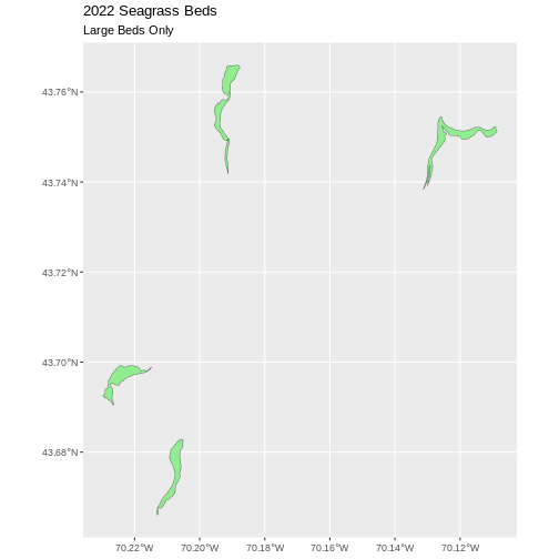
There are four features in our large beds subset. But we don’t have
any more information than that they are large. Let’s adjust the colors
used in our plot. If we have 4 features in our vector object, we can
plot each using a unique color by assigning a column name to the color
aesthetic (fill =). We use the syntax
aes(fill = ) to do this. Let’s look at
Cover_Pct to differentiate sparse from dense beds.
R
ggplot() +
  geom_sf(data = large_beds, aes(fill = Cover_Pct)) +
  labs(color = 'Percent Cover of Seagrass') +
  ggtitle("2022 Seagrass Beds", subtitle = "Sparse Beds Only") +
  coord_sf()
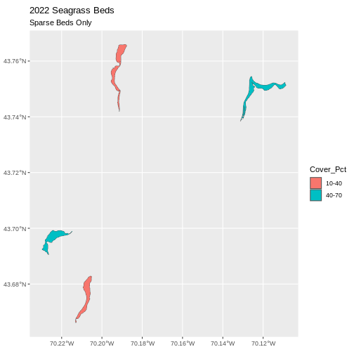
Now, we see that there are in some dense and some sparse beds that are big.
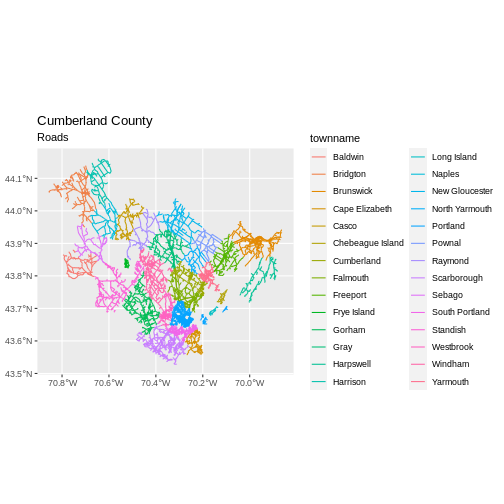
First we will save an object with only the roads in Cumberland:
R
cumberland_roads <- roads_maine %>%
  filter(cntyname == "Cumberland")
Let’s check how many features there are in this subset:
R
nrow(cumberland_roads)
OUTPUT
[1] 18246Now let’s plot that data:
R
ggplot() +
  geom_sf(data = cumberland_roads,
          aes(color = townname),
          size = 1.5) +
  ggtitle("Cumberland County", subtitle = "Roads") +
  coord_sf()
Challenge: Subset Spatial Polygon Objects and Plotting
Are dense beds large or small? From seagrass_casco_2022,
subset out only the dense beds - Cover_Pct == "70-100".
How many dense beds are there?
What is the distribution of their size?
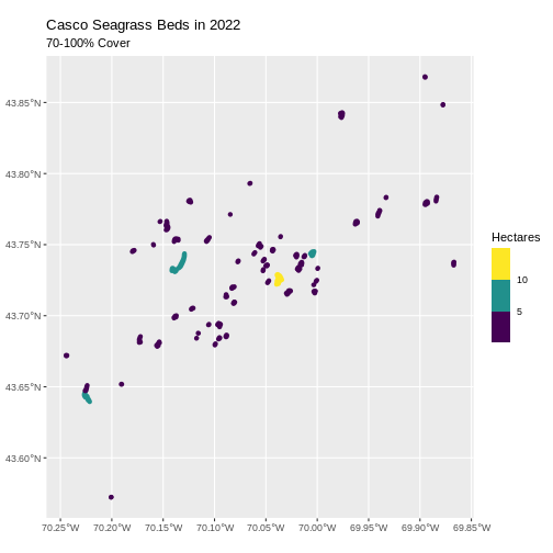
Plotthem . To make it interesting, set the color (not the fill) to map to
Hectaresso that we can see where big dense beds exist. To further assist with this A) you will need to setlinewidth = 2, as otherwise you won’t be able to see the beds well and B) you’ll need to use a binned color scale, like we did with rasters. I’m a fan ofscale_color_viridis_b()here, but also feel free to try some options fromscale_color_fermenter()or play with then.binsargument.
- First we will save an object with only the stone wall lines and check the number of features:
R
dense_beds <- seagrass_casco_2022 %>%
  filter(Cover_Pct == "70-100")

nrow(dense_beds)
OUTPUT
[1] 79- Is the distribution different than the size of all beds? Let’s see.
R
ggplot(data = dense_beds,
       aes(x = Hectares)) +
  geom_histogram(bins = 50)
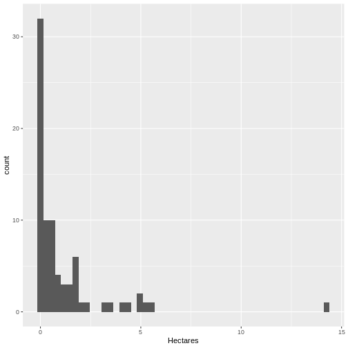
It’s roughly similar, although there seem to be more mid-size beds.
- Last, we can plot the data:
R
ggplot() +
  geom_sf(data = dense_beds, aes(color = Hectares),
          linewidth = 2) +
  ggtitle("Casco Seagrass Beds in 2022", subtitle = "70-100% Cover") +
  coord_sf() +
  scale_color_viridis_b()
Customize Plots
In the examples above, ggplot() automatically selected
colors for each line based on a default color order. If we don’t like
those default colors, we can create a vector of colors - one for each
feature.
First we will check how many unique levels our factor has:
R
unique(seagrass_casco_2022$Cover_Pct)
OUTPUT
[1] "0-10" "40-70" "70-100" "10-40" Then we can create a palette of four colors, one for each feature in our vector object.
R
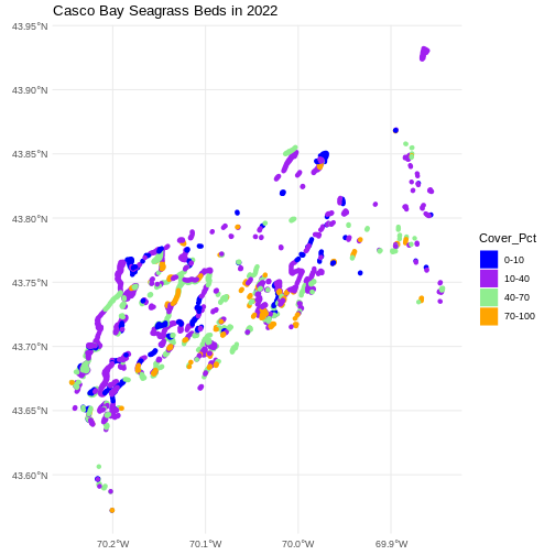
bed_colors <- c("blue", "purple", "lightgreen", "orange")
We can tell ggplot to use these colors when we plot the
data.
R
ggplot() +
  geom_sf(data = seagrass_casco_2022,
          aes(color = Cover_Pct, fill = Cover_Pct),
          linewidth = 2) +
  scale_color_manual(values = bed_colors) +
  scale_fill_manual(values = bed_colors) +
  ggtitle("Casco Bay Seagrass Beds in 2022") +
  coord_sf() +
  theme_minimal()
Improve Our Plot Legend
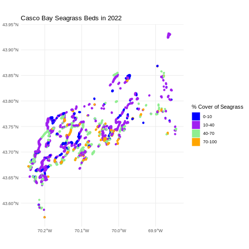
Let’s improve the legend of our plot. We’ve already created a
legenend for Cover_Pct by default. Let’s start by making
the title be readable using labs() to give it titles. Note,
color and fill must have the same title, otherwise the legend
splits.
R
ggplot() +
  geom_sf(data = seagrass_casco_2022,
          aes(color = Cover_Pct, fill = Cover_Pct),
          linewidth = 2) +
  scale_color_manual(values = bed_colors) +
  scale_fill_manual(values = bed_colors) +
  labs(color = '% Cover of Seagrass', fill = "% Cover of Seagrass") +
  ggtitle("Casco Bay Seagrass Beds in 2022") +
  coord_sf() +
  theme_minimal()
We can change the appearance of our legend by manually setting
different parameters using the theme() function.
-
legend.title: change the legend title font size -
legend.text: change the legend text font size -
legend.box.background: add an outline box -
legend.position: where you want the legend. Options include “none”, “left”, “right”, “bottom”, “top”, or two-element numeric vector.
Note, some of these will need an element_*() function.
To dig deep deep into plot customization, see ?theme
R
ggplot() +
  geom_sf(data = seagrass_casco_2022,
          aes(color = Cover_Pct, fill = Cover_Pct),
          linewidth = 2) +
  scale_color_manual(values = bed_colors) +
  scale_fill_manual(values = bed_colors) +
  labs(color = '% Cover of Seagrass', fill = "% Cover of Seagrass") +
  ggtitle("Casco Bay Seagrass Beds in 2022") +
  coord_sf() +
  theme_minimal(base_size = 14)  +
  theme(legend.title = element_text(size = 14),
        legend.text = element_text(size = 12),
        legend.box.background = element_rect(linewidth = 1),
        legend.position = "bottom")
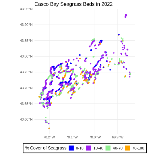
theme_minimal() here is a premade ggplot2 theme. You can
also use theme() to make your own customized themes.
Challenge: Visualizing Change
Create a similar plot from the 2023 data. There are some differences.
Cover_Pct is slightly different. You’ll have to filter out
the "0%“` beds in order to use the identical color palette
(a good idea in order to see change).
Do you see differences between 2013 and 2022?
First we explore load and filter the data.
R
seagrass_casco_2013 <-
  st_read("data/maine_gov_seagrass/MaineDEP_Casco_Bay_Eelgrass_2013/") |>
  filter(Cover_Pct != "0%")
OUTPUT
Reading layer `MaineDEP_Casco_Bay_Eelgrass_2013' from data source
  `/home/runner/work/r-raster-vector-geospatial/r-raster-vector-geospatial/site/built/data/maine_gov_seagrass/MaineDEP_Casco_Bay_Eelgrass_2013'
  using driver `ESRI Shapefile'
Simple feature collection with 1056 features and 7 fields
Geometry type: POLYGON
Dimension:     XY
Bounding box:  xmin: -70.2477 ymin: 43.5896 xmax: -69.84402 ymax: 43.93288
Geodetic CRS:  WGS 84
Then, honestly, we can re-use the same plotting code as above.
R
ggplot() +
  geom_sf(data = seagrass_casco_2013,
          aes(color = Cover_Pct, fill = Cover_Pct),
          linewidth = 2) +
  scale_color_manual(values = bed_colors) +
  scale_fill_manual(values = bed_colors) +
  labs(color = '% Cover of Seagrass', fill = "% Cover of Seagrass",
       title = "Casco Bay Seagrass Beds in 2013") +
  coord_sf() +
  theme_minimal(base_size = 14)  +
  theme(legend.title = element_text(size = 14),
        legend.text = element_text(size = 12),
        legend.box.background = element_rect(linewidth = 1),
        legend.position = "bottom")
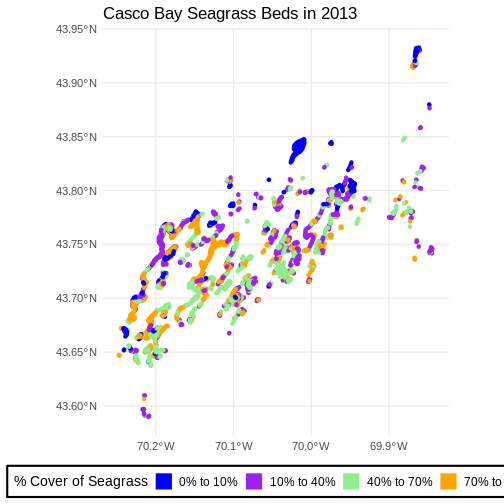
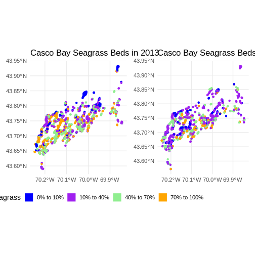
Flip back and forth between the two maps. Qualitatively, it looks like beds are less dense.
Data Tip
You can plot multiple plot panels next to each other using the patchwork library.
R
library(patchwork)

beds_2013 <- ggplot() +
  geom_sf(data = seagrass_casco_2013,
          aes(color = Cover_Pct, fill = Cover_Pct),
          linewidth = 2) +
  scale_color_manual(values = bed_colors) +
  scale_fill_manual(values = bed_colors) +
  labs(color = '% Cover of Seagrass', fill = "% Cover of Seagrass",
       title = "Casco Bay Seagrass Beds in 2013") +
  coord_sf() +
  theme_minimal(base_size = 14)

beds_2022 <- ggplot() +
  geom_sf(data = seagrass_casco_2022,
          aes(color = Cover_Pct, fill = Cover_Pct),
          linewidth = 2) +
  scale_color_manual(values = bed_colors) +
  scale_fill_manual(values = bed_colors) +
  labs(title = "Casco Bay Seagrass Beds in 2022") +
  coord_sf() +
  theme_minimal(base_size = 14)

# the patchwork - note removing one legend for ease of viz
# as they are the same but different text
(beds_2013 & theme(legend.position = 'bottom')) +
  (beds_2022 & theme(legend.position = "none"))
Content from Plot Multiple Vector Layers
Last updated on 2024-03-12 | Edit this page
Estimated time: 60 minutes
WARNING
Warning in
download.file("https://www.naturalearthdata.com/http//www.naturalearthdata.com/download/110m/physical/ne_110m_graticules_all.zip",
: cannot open URL
'https://www.naturalearthdata.com/http//www.naturalearthdata.com/download/110m/physical/ne_110m_graticules_all.zip':
HTTP status was '500 Internal Server Error'
ERROR
Error in download.file("https://www.naturalearthdata.com/http//www.naturalearthdata.com/download/110m/physical/ne_110m_graticules_all.zip", : cannot open URL 'https://www.naturalearthdata.com/http//www.naturalearthdata.com/download/110m/physical/ne_110m_graticules_all.zip'Overview
Questions
- How can I make different vecotr layers line up?
- How can I plot multiple forms of vector data together?
Objectives
- Plot multiple vector layers in the same plot.
- Apply custom symbols to spatial objects in a plot.
- Create a multi-layered plot with raster and vector data.
Things You’ll Need To Complete This Episode
See the lesson homepage for detailed information about the software, data, and other prerequisites you will need to work through the examples in this episode.
This episode builds upon the previous episode to work with vector layers in R and explore how to plot multiple vector layers. It also covers how to plot raster and vector data together on the same plot.
Load the Data
To work with vector data in R, we can use the sf
library. We will also be using ggplot2 and some
dplyr. Let’s start by loading them.
R
library(ggplot2)
library(dplyr)
library(sf)
We are going to plot the 2022 Casco Bay Seagrass Beds, but, include some coastline for context. We will also add layers of information along the way. To start with, let’s load up the seagrass beds, the AOI for Casco, and a shapefile of counties in Maine.
R
aoi_boundary_casco <- st_read(
  "data/maine_gov_maps/casco_aoi/casco_bay_aoi.shp")

seagrass_casco_2022 <- st_read(
  "data/maine_gov_seagrass/MaineDEP_Casco_Bay_Seagrass_2022/MaineDEP_Casco_Bay_Seagrass_2022.shp")

maine_borders <- st_read(
  "data/maine_gov_maps/Maine_State_Boundary_Polygon_Feature/Maine_State_Boundary_Polygon_Feature.shp")
Making Sure Layers Match in Extent
One of the beautiful things about ggplot2 is that we’re
going to be able to just add layers together to make a nice plot. Our
goal here is to plot seagrass beds with a coastline bordering them, so
we can see how they line up around islands. However, we have a small
problem. Let’s compare the extent of our objects using
st_bbox().
R
st_bbox(aoi_boundary_casco)
OUTPUT
    xmin     ymin     xmax     ymax
-70.2528  43.5834 -69.8387  43.9439
R
st_bbox(seagrass_casco_2022)
OUTPUT
     xmin      ymin      xmax      ymax
-70.24464  43.57213 -69.84399  43.93221
R
st_bbox(maine_borders)
OUTPUT
     xmin      ymin      xmax      ymax
-71.08392  42.97703 -66.94942  47.45986
While the first two are close - indeed, the AOI was made from the
seagrass polygons extent - the state of Maine is huge relative to Casco
Bay. We need to crop that shapefile down to just the
area we want to plot. Fortunately, sf features a function
called st_crop() which will crop a large vector file down
to the size of the extent of a smaller vector file. So if we just want
the Casco Coastline, we can crop maine_borders down to the
size of the aoi_boundary_casco vector file.
R
casco_coastline <- st_crop(maine_borders, aoi_boundary_casco)
ERROR
Error in wk_handle.wk_wkb(wkb, s2_geography_writer(oriented = oriented, : Loop 0 is not valid: Edge 47287 has duplicate vertex with edge 47329This does not always go well with data sets from the wild. Without
getting too deep into it, vector files (particularly polygons) can have
a variety of issues in them which make them invalid. To fix this, we
need to make them valid before cropping with
st_make_valid(). Odd, but, this is incredibly common.
R
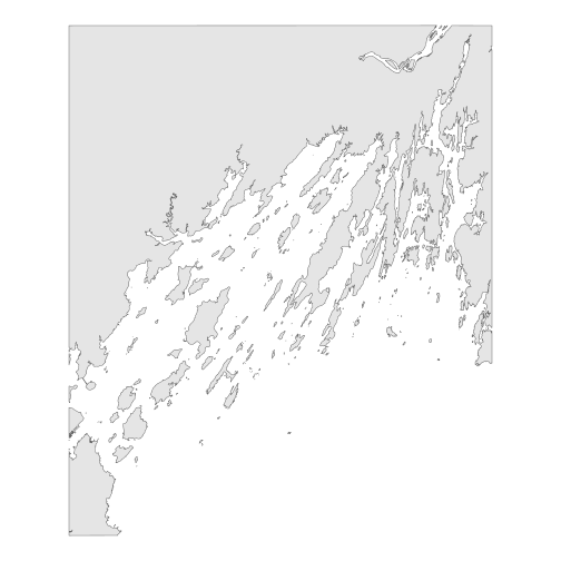
casco_coastline <- st_crop(maine_borders |> st_make_valid(),
                           aoi_boundary_casco)

ggplot() +
  geom_sf(data = casco_coastline) +
  coord_sf() +
  theme_void()
R
roads_maine <- st_read("data/maine_gov_maps/MaineDOT_Public_Roads/MaineDOT_Public_Roads.shp")
OUTPUT
Reading layer `MaineDOT_Public_Roads' from data source
  `/home/runner/work/r-raster-vector-geospatial/r-raster-vector-geospatial/site/built/data/maine_gov_maps/MaineDOT_Public_Roads/MaineDOT_Public_Roads.shp'
  using driver `ESRI Shapefile'
Simple feature collection with 100669 features and 30 fields
Geometry type: LINESTRING
Dimension:     XY
Bounding box:  xmin: -71.04662 ymin: 43.06728 xmax: -66.95202 ymax: 47.35999
Geodetic CRS:  WGS 84
R
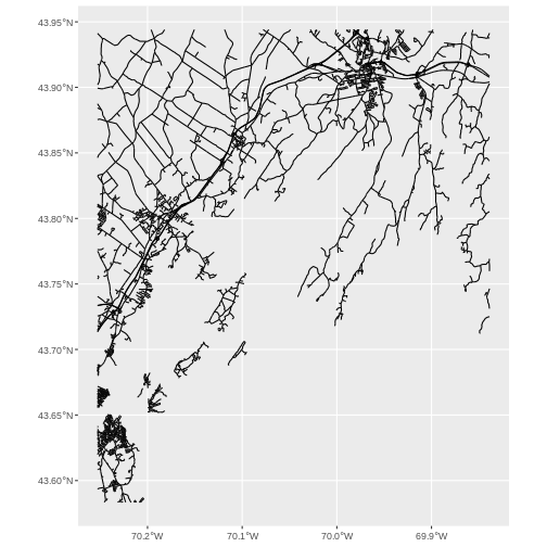
roads_casco <- st_crop(roads_maine, aoi_boundary_casco)

ggplot() +
  geom_sf(data = roads_casco)
Lovely! Now let’s start bringing seagrass in.
Plotting Multiple Vector Layers
In the previous episode, we learned how to plot information from a single vector layer and do some plot customization including adding a custom legend. However, what if we want to create a more complex plot with many vector layers and unique symbols that need to be represented clearly in a legend?
Now, let’s create a plot that combines our seagrass beds
(seagrass_casco_2022), the coastline
(casco_coastline) and roads (roads_maine)
spatial objects. We will need to build a custom legend as well.
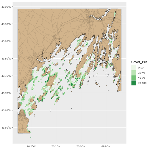
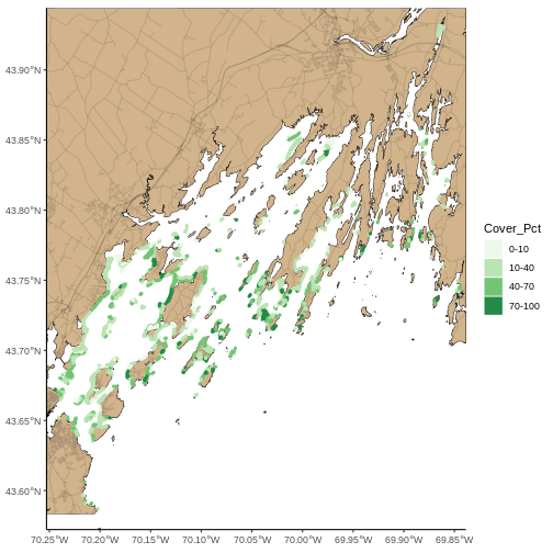
To begin, we will create a plot with the coastline as the base layer with a tan fill and a black outline. We will add on top roads, but with alpha = 0.1 so they are faint. Last, we will layer seagrass beds on top with color and fill as percent cover and a linewidth of 1.3. We will save it as an object so we can make small changes from here on out.
R
seagrass_map <- ggplot() +
  geom_sf(data = casco_coastline, fill = "tan", color = "black") +
  geom_sf(data = roads_casco, alpha = 0.1) +
  geom_sf(data = seagrass_casco_2022,
          mapping = aes(color = Cover_Pct,
                        fill = Cover_Pct),
          linewidth = 1.3) +
  scale_color_brewer(palette = "Greens") +
  scale_fill_brewer(palette = "Greens")

seagrass_map
This looks OK, but, let’s dial things up a bit. Let’s
- Eliminate the gap around the plot with an argument
expand = FALSEtocoord_sf(). - Give it a cleaner theme with
theme_classic() - Give the map a name and the fill/color legend a name.
- Use
theme()to make it more ocean-y with a
We can start by making the plot cleaner and eliminating the gap (1 & 2)
R
seagrass_map <- seagrass_map +
  coord_sf(expand = FALSE) +
  theme_classic()

seagrass_map
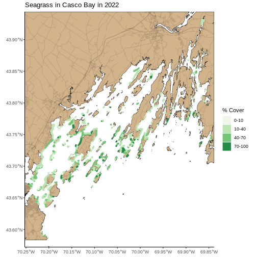
Now lets adjust the legend titles by using labs().
R
seagrass_map <- seagrass_map +
  labs(color = "% Cover", fill = "% Cover",
       title = "Seagrass in Casco Bay in 2022")

seagrass_map
Last, we can use theme() to add a light blue background
and rotate the X axis. We will save this as an object, so we don’t need
to type more as we make further modifications.
R
seagrass_map <- seagrass_map  +
  theme(panel.background = element_rect(fill = "lightblue"),
        axis.text.x = element_text(angle = 45, hjust = 1))

seagrass_map
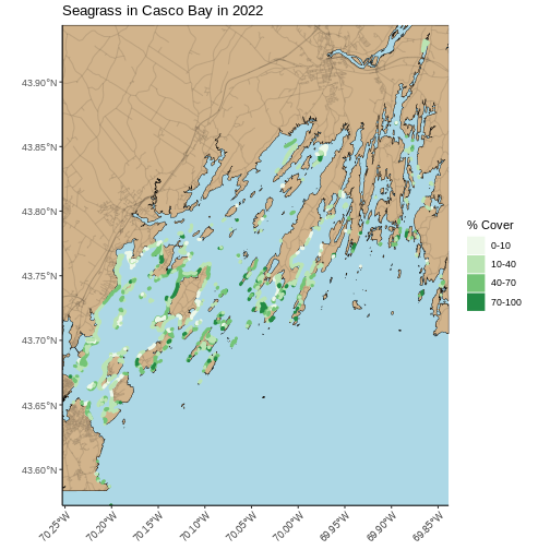
Zooming In
This map looks great, but, there’s a lot of data here. While it can provide a great big-picture overview, it’s hard to see more small-scale features. There are two solutions to this. The first is plotting the map zoomed in to an area of interest. You can get your AOI either by eyeballing the corner coordinates (x and y min and max) from the plot itself, or use something like https://maps.google.com and right click to get point coordinates.
Using the later method, here, for example, is the area around Mackworth Island.
R
seagrass_map +
  coord_sf(xlim = c(-70.24768051612979, -70.19432151530208),
           ylim = c(43.66353031177649, 43.714022044471584),
           expand = FALSE)
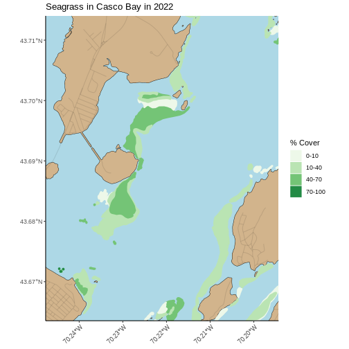
The second answer is an interactive map with leaflet. This is
slightly more challenging to implement, but very similar to what we did
with rasters before. We will start by making a color palette for the
map. We can use colorFactor() as we have discrete classes
here.
R
library(leaflet)

seagrass_pal <- colorFactor(palette = "Greens",
                         domain = seagrass_casco_2022$Cover_Pct)
From here, we can build a leaflet map. Let’s use
addProviderTiles("Stadia.AlidadeSmooth") for a very neutral
background. We add sf polygons using
addPolygons(). For this, we need to think about the what is
creating polygon borders and the fill. We will set
stroke = FALSE so we don’t have to worry about the border
(too many more argument) and instead use our palette - which is now a
function to be evaluated with ~ and set a
fillOpacity to 1, for fully opaque.
R
leaflet() |>
 addProviderTiles("Stadia.AlidadeSmooth") |>
  addPolygons(data = seagrass_casco_2022,
              fillColor = ~seagrass_pal(Cover_Pct),
              fillOpacity = 1,
              stroke = FALSE)
Note, you can recreate what you did with the ggplot2
above just using the sf objects. We’ll need to invoke one
trick from the leaflet.extras package to get that blue
background.
R
library(leaflet.extras)

leaflet() |>
  addPolygons(data = casco_coastline,
              fillColor = "tan",
              fillOpacity = 1,
              stroke = FALSE) |>
  addPolylines(data = roads_casco,
               color = "black",
               opacity = 0.1,
               weight = 1) |>
  addPolygons(data = seagrass_casco_2022,
              fillColor = ~seagrass_pal(Cover_Pct),
              fillOpacity = 1,
              stroke = FALSE) |>
  addPolygons(data = aoi_boundary_casco,
              color = "black",
              fillOpacity = 0) |>
  setMapWidgetStyle(list(background= "lightblue")) |>
  addLegend(pal = seagrass_pal,
            values = seagrass_casco_2022$Cover_Pct,
            title = "% Cover Seagrass")
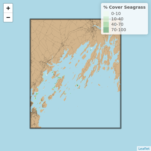
Challenge: Let’s Part Like it’s 1997… er, 1993-1994
The earliest seagrass datat available from Maine’s Geolibrary is their 1997 State-Wide Data aggregated from photography from 1992 - 1997. Load up the ESRI
shapefilefromdata/maine_gov_seagrass/MaineDMR_-_Eelgrass-1997-shpand do a quick visualization showing where was surveyed when.Crop it down to Casco Bay and make a plot showing the area around Mackworth Island. Make sure your title reflects what years are being represented. While there is a cover classification (from 0-5) based on percent cover, the metadata doesn’t have the lineup. Still, qualitatively, how does this compare to 2022? Use whatever technique you’d like to visualize this small area. Note,
COVERis continuous, so to make it into distinct classes you will needas.character(COVER)in your code.
- First we need to load in the data. Let’ see how many years are here.
R
seagrass_1997 <- st_read("data/maine_gov_seagrass/MaineDMR_-_Eelgrass-1997-shp/MaineDMR_-_Eelgrass.shp")
OUTPUT
Reading layer `MaineDMR_-_Eelgrass' from data source
  `/home/runner/work/r-raster-vector-geospatial/r-raster-vector-geospatial/site/built/data/maine_gov_seagrass/MaineDMR_-_Eelgrass-1997-shp/MaineDMR_-_Eelgrass.shp'
  using driver `ESRI Shapefile'
Simple feature collection with 7519 features and 10 fields
Geometry type: POLYGON
Dimension:     XY
Bounding box:  xmin: -70.82449 ymin: 43.05945 xmax: -66.98462 ymax: 45.11247
Geodetic CRS:  WGS 84
R
# what are the names
names(seagrass_1997)
OUTPUT
 [1] "OBJECTID_1" "OBJECTID"   "COVER"      "LOCATION"   "ACRES"
 [6] "HECTARES"   "Year97"     "GlobalID"   "Shape__Are" "Shape__Len"
[11] "geometry"
R
# what are the unique years
unique(seagrass_1997$Year97)
OUTPUT
[1] 1993 1994 1997 1996 1992 1995Then, we can visualize.
R
ggplot() +
  geom_sf(data = seagrass_1997,
          aes(color = Year97, fill = Year97)) +
  scale_color_viridis_c() +
  scale_fill_viridis_c()
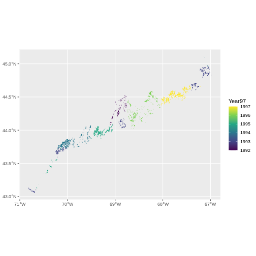
- For the second piece, first, we need to crop to Casco Bay and check what years this data consists of.
R
seagrass_casco_1997 <- st_crop(seagrass_1997 |> st_make_valid(),
                              aoi_boundary_casco)

unique(seagrass_casco_1997$Year97)
OUTPUT
[1] 1994 1993With the cropped polygons, we can make a map akin to what we did above for 2022. We can even re-use our code, but with a few small modifications for a different data set and a different cover type.
R
ggplot() +
  geom_sf(data = casco_coastline, fill = "tan", color = "black") +
  geom_sf(data = roads_casco, alpha = 0.1) +
  geom_sf(data = seagrass_casco_1997,
          mapping = aes(color = as.character(COVER),
                        fill = as.character(COVER)),
          linewidth = 1.3) +
  scale_color_brewer(palette = "Greens") +
  scale_fill_brewer(palette = "Greens") +
  theme_classic() +
  labs(color = "Cover Class", fill = "Cover Class",
       title = "Seagrass in Casco Bay in 1993 and 1994") +
  coord_sf(xlim = c(-70.24768051612979, -70.19432151530208),
           ylim = c(43.66353031177649, 43.714022044471584),
           expand = FALSE) +
  theme(panel.background = element_rect(fill = "lightblue"),
        axis.text.x = element_text(angle = 45, hjust = 1))
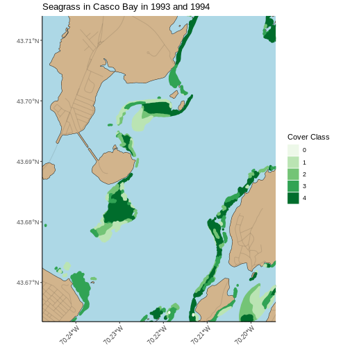
While we cannot know how the beds compare exactly, given that we do not know how the Cover Class maps to % Cover, it appears that many of the beds in 1993 and 1994 are at the highest class of cover, while in 2022 they are at the high-middle.
Content from Handling Spatial Projection & CRS
Last updated on 2024-03-12 | Edit this page
Estimated time: 60 minutes
WARNING
Warning in
download.file("https://www.naturalearthdata.com/http//www.naturalearthdata.com/download/110m/physical/ne_110m_graticules_all.zip",
: cannot open URL
'https://www.naturalearthdata.com/http//www.naturalearthdata.com/download/110m/physical/ne_110m_graticules_all.zip':
HTTP status was '500 Internal Server Error'
ERROR
Error in download.file("https://www.naturalearthdata.com/http//www.naturalearthdata.com/download/110m/physical/ne_110m_graticules_all.zip", : cannot open URL 'https://www.naturalearthdata.com/http//www.naturalearthdata.com/download/110m/physical/ne_110m_graticules_all.zip'Overview
Questions
- How do I work with data sets that are in different projections?
Objectives
- Examine objects with different CRSs in the same plot.
- Reproject a raster and a vector layer in R.
- Plot vector and raster layers in the same plot.
Things You’ll Need To Complete This Episode
See the lesson homepage for detailed information about the software, data, and other prerequisites you will need to work through the examples in this episode.
Projection in R
In an earlier episodes we learned how to layer multiple vector data types. These principles extend to layering in raster data. When combining multiple data sources, particularly from different agencies or research efforts, we often find that they do not have the same Coordinate Reference System. This can be true of combining multiple vectors or rasters, or both.
We will apply our skills learned thus far to create maps that combine
both the coastline of Casco Bay (casco_coastline) with SST
data from 2022 (b10_casco_2022) and seagrass data
(seagrass_casco_2022). We will learn how to map vector data
sources that are in different CRSs and thus don’t line up on a map.
Load the Data
We will continue to use the sf and terra
packages in this episode as well as others from previously.
R
library(terra)
library(sf)
library(ggplot2)
library(tidyterra)
library(dplyr)
We will continue to work with the two ESRI shapefiles
that we loaded in the previously as well
as some Sea Surface Temperature data from our raster lessons.
R
# Casco Bay SST from Sept 9, 2022
b10_casco_2022 <- rast(
  "data/landsat_casco/b10_cropped/LC08_L2SP_011030_20220909_20220914_02_T1_ST_B10.TIF")

# Seagrass beds in 2022
seagrass_casco_2022 <- st_read(
  "data/maine_gov_seagrass/MaineDEP_Casco_Bay_Seagrass_2022/MaineDEP_Casco_Bay_Seagrass_2022.shp")

# Casco Coastline
casco_coastline <- st_read(
  "data/maine_gov_maps/Maine_State_Boundary_Polygon_Feature/Maine_State_Boundary_Polygon_Feature.shp") |>
  st_make_valid() |>
  st_crop(seagrass_casco_2022)
Working With Spatial Data From Different Sources
We often need to gather spatial datasets from different sources and/or data that cover different spatial extents. These data are often in different Coordinate Reference Systems (CRSs).
Some reasons for data being in different CRSs include:
- The data are stored in a particular CRS convention used by the data provider (for example, a government agency).
- The data are stored in a particular CRS that is customized to a region. For instance, many states in the US prefer to use a State Plane projection customized for that state.
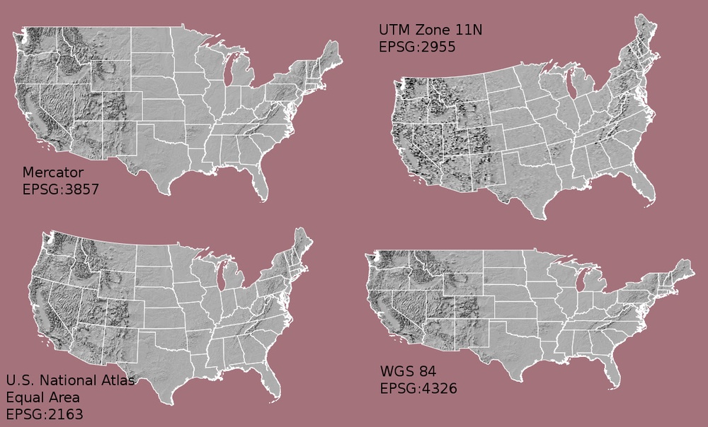
Notice the differences in shape associated with each different projection. These differences are a direct result of the calculations used to “flatten” the data onto a 2-dimensional map. Often data are stored purposefully in a particular projection that optimizes the relative shape and size of surrounding geographic boundaries (states, counties, countries, etc).
In this episode we will learn how to identify and manage spatial data in different projections. We will learn how to reproject the data so that they are in the same projection to support plotting / mapping. Note that these skills are also required for any geoprocessing / spatial analysis. Data need to be in the same CRS to ensure accurate results.
Inspecting CRS
To begin, how different are these two data sources? We can inspect their respective Coordinate Reference Systems to see.
R
crs(b10_casco_2022, proj = TRUE)
OUTPUT
[1] "+proj=utm +zone=19 +datum=WGS84 +units=m +no_defs"R
crs(casco_coastline, proj = TRUE)
OUTPUT
[1] "+proj=longlat +datum=WGS84 +no_defs"R
# st_crs(casco_coastline)$proj4string #this also works
Our project string for b10_casco_2022 specifies the UTM
projection as follows:
+proj=utm +zone=19 +datum=WGS84 +units=m +no_defs
- proj=utm: the projection is UTM, UTM has several zones.
- zone=19: the zone is 19
- datum=WGS84: the datum WGS84 (the datum refers to the 0,0 reference for the coordinate system used in the projection)
- units=m: the units for the coordinates are in METERS.
- no_defs: nothing is used from detault files.
Note that the zone is unique to the UTM projection. Not
all CRSs will have a zone.
For casco_coastline
Our project string for casco_coastline specifies the
lat/long projection as follows:
+proj=longlat +datum=WGS84 +no_defs
- proj=longlat: the data are in a geographic (latitude and longitude) coordinate system
- datum=WGS84: the datum WGS84 (the datum refers to the 0,0 reference for the coordinate system used in the projection)
- no_defs: nothing is used from detault files.
Note that there are no specified units above. This is because this geographic coordinate reference system is in latitude and longitude which is most often recorded in decimal degrees.
Sometimes you will also see ellps=WGS84: the ellipsoid (how the earth’s roundness is calculated) is WGS84.
The projections are very different. Refer to UTM versus UTM in the figure of the US above.
Do We Need to Reproject?
We can begin by trying to plot these datasets together. One of the
nice things about tidyterra and how ggplot2
works with sf objects is that it projects them to the same
CRS. So, if we try and plot these data sources together:
R
ggplot() +
  geom_spatraster(data = b10_casco_2022) +
  geom_sf(data = casco_coastline) +
  scale_fill_viridis_c()
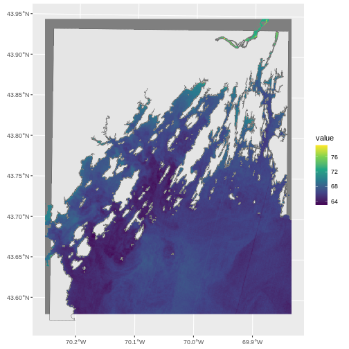
This looks pretty good. Leaflet looks good as well.
R
library(leaflet)

leaflet() |>
  addPolygons(data = casco_coastline,
              fill = "white", weight = 1,
              color = "black") |>
  addRasterImage(b10_casco_2022)
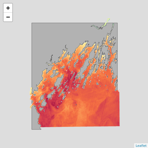
But, note two things. First, not every plotting algorithm will work.
For example if we went old school and used plot() with
add=TRUE to add a layer, this would have failed. Here we
see if putting a different layer down as the base.
R
par(mfrow = c(1,2))

plot(b10_casco_2022, main = "SST First")
plot(casco_coastline$geometry, add = TRUE)

plot(casco_coastline$geometry, main = "Coastline First", axes = TRUE)
plot(b10_casco_2022, add = TRUE)
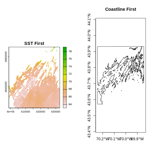
R
par(mfrow = c(1,1))
Where did the other layer go? The axes give away that it’s a projection problem.
Second, in both of these, the borders and the raster don’t line up. So we want to line up extents. This is an aesthetic concern, but can be a big one - particularly if we were doing operations other than plotting. We need to crop one data set by the other.
Cropping and CRS
Cropping involves cutting off one part of an object to match another.
It is one of the operations we use to subset data spatially. We can also
extend objects to add rows or columns or mask out parts of an object. In
this case, let’s crop b10_casco_2022 so that we get rid of
that NA edge. After, we can crop the the coastline in order to eliminate
that weird hang-on piece of coast at the bottom of the maps.
As we are cropping a terra SpatRaster
object, we will use crop() which takes an input raster and
then an object with an extent to crop it to.
R
b10_casco_2022_cropped <- crop(b10_casco_2022,
                               casco_coastline)
ERROR
Error: [crop] extents do not overlapWell that’s odd. What are their extents?
R
ext(b10_casco_2022)
OUTPUT
SpatExtent : 398865, 432705, 4825935, 4866405 (xmin, xmax, ymin, ymax)R
ext(casco_coastline)
OUTPUT
SpatExtent : -70.244637867776, -69.843989726984, 43.5721328168498, 43.9322969014411 (xmin, xmax, ymin, ymax)Those are very different numbers due to their different CRS’s that we looked at above. This means, we will have to REPROJECT one of the two objects in order to crop it successfully, and then work in a common CRS.
Which data source should I reproject?
Projection works on a pixel by pixel basis. That means that for every pixel in your data, your computer will be doing work. As your data sets increase in size, projection can be computationally very expensive. In these cases, think about which layer will process faster. Often, it’s faster to project vector data, as it contains a tiny fraction of the points that are found in a raster data set.
While we can write a long CRS string, it’s easier to just take it
from an object or specify what’s called an EPSG code from epsg.org. We can see those codes
using crs() from terra with
describe = TRUE
R
crs(casco_coastline, describe = TRUE)
OUTPUT
    name authority code area         extent
1 WGS 84      EPSG 4326 <NA> NA, NA, NA, NA
From this we can see the EPSG code is 4326.
For the SST data…
R
crs(b10_casco_2022, describe = TRUE)
OUTPUT
                   name authority  code
1 WGS 84 / UTM zone 19N      EPSG 32619
                                                                                                                                                                                                                                                                                                                         area
1 Between 72°W and 66°W, northern hemisphere between equator and 84°N, onshore and offshore. Aruba. Bahamas. Brazil. Canada - New Brunswick (NB); Labrador; Nunavut; Nova Scotia (NS); Quebec. Colombia. Dominican Republic. Greenland. Netherlands Antilles. Puerto Rico. Turks and Caicos Islands. United States. Venezuela
           extent
1 -72, -66, 84, 0
the EPSG code is 32619.
Regardless, we can reproject the raster to the same projection as the coastline.
R
b10_casco_2022_4326 <- project(b10_casco_2022,
                               crs(casco_coastline))

b10_casco_2022_4326
OUTPUT
class       : SpatRaster
dimensions  : 1159, 1343, 1  (nrow, ncol, nlyr)
resolution  : 0.0003176554, 0.0003176554  (x, y)
extent      : -70.26025, -69.83364, 43.57953, 43.94769  (xmin, xmax, ymin, ymax)
coord. ref. : lon/lat WGS 84 (EPSG:4326)
source(s)   : memory
name        : SST_F_20220909
min value   :       63.06477
max value   :       79.34391
Note the difference in information about the projection (and EPSG code).
To transform sf vector data, we would have used the
function st_transform().
Proj4 & CRS Resources
- Official PROJ library documentation
- More information on the proj4 format.
- A fairly comprehensive list of CRSs by format.
- To view a list of datum conversion factors type:
sf_proj_info(type = "datum")into the R console. However, the results would depend on the underlying version of the PROJ library.
Cropping and Plotting
Now we can crop. We will first crop the SST raster to the coastline in order to get rid of the NA area in the raster.
R
b10_casco_2022_4326_cropped <- crop(b10_casco_2022_4326,
                                    casco_coastline)
Then we will crop the coastline to the cropped raster in order to get rid of that little bit of coast on the southern end.
R
casco_coastline_cropped <- st_crop(casco_coastline,
                                   b10_casco_2022_4326_cropped)
Let’s plot it and see if all of the effort was worth it!
R
ggplot() +
  geom_spatraster(data = b10_casco_2022_4326_cropped) +
  geom_sf(data = casco_coastline_cropped, fill = "tan") +
  scale_fill_viridis_c() +
  labs(fill = "SST (F)") +
  coord_sf(expand = FALSE)
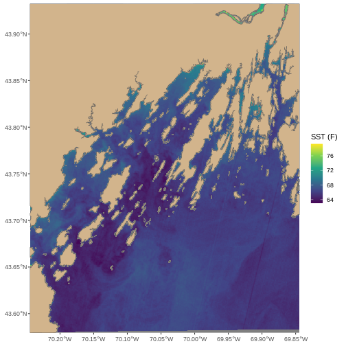
Summary: When CRS Attacks
The workflow outlined here, while in depth, is actually relatively simple. When you have two or more spatial data sets that you want to line up in terms of extent and projection.
- Determine if they actually differ in projection. If not, skip to 2.
- Reproject the smaller data source to the CRS of the larger one (if size is a concern).
- Crop back and forth to line up extents.
- Plot!
Challenge - Show us the temperature of seagrass beds
Let’s combine our SST and Seagrass data from 2022 to see if seagrasses are in warm places around Mackworth. Let’s start by making a Macworth Island AOI. We will do this by making a bounding box, and then turning it into an sf object.
R
mackworth_aoi <- st_bbox(c(xmin = -70.24768051612979,
                           xmax = -70.19432151530208,
                           ymin = 43.66353031177649,
                           ymax = 43.714022044471584),
                         crs = 4326) |>
  st_as_sfc()
Reproject the AOI and seagrass data to the same projection as the SST raster. Note, to get the CRS in a format
sfrecognizes, usest_crs(). We can leave out the coast.Crop everything to the Mackworth AOI. Note,
sfusesst_crop()whileterrausescrop.Plot! Try leaving seagrass polygons with an
NAfill to see the temperature inside and outside of the beds. As land is NA here, you can use thena.valueargument to yourscale_fill_*()to make the land tan.
- Reprojection
R
seagrass_casco_2022_32619 <- st_transform(seagrass_casco_2022,
                                          st_crs(b10_casco_2022))

mackworth_32619 <- st_transform(mackworth_aoi,
                              st_crs(b10_casco_2022))
- Cropping
R
seagrass_casco_2022_32619_mackworth <- st_crop(seagrass_casco_2022_32619,
                                               mackworth_32619)

b10_casco_2022_mackworth <- crop(b10_casco_2022,
                                 mackworth_32619)
- Plot!
R
ggplot() +
  geom_spatraster(data = b10_casco_2022_mackworth) +
  geom_sf(data = seagrass_casco_2022_32619_mackworth,
          color = "black",
          linewidth = 1,
          fill = NA) +
  scale_fill_viridis_c(na.value = "tan") +
  coord_sf(expand = FALSE)
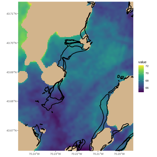
Looks like they are not in the warmest spots, but generally waters that in this Landsat scene were a bit cooler.
Key Points
- Multi-layered plots can combine vector and raster data sets.
-
ggplot2automatically converts all objects in a plot to the same CRS. - Still be aware of the CRS and extent for each object.
-
project()andst_transform()will reproject raster and vector data. -
crop()andst_crop()will crop raster and vector data.
Content from Convert from .csv to a Vector Layer
Last updated on 2024-03-12 | Edit this page
Estimated time: 60 minutes
WARNING
Warning in
download.file("https://www.naturalearthdata.com/http//www.naturalearthdata.com/download/110m/physical/ne_110m_graticules_all.zip",
: cannot open URL
'https://www.naturalearthdata.com/http//www.naturalearthdata.com/download/110m/physical/ne_110m_graticules_all.zip':
HTTP status was '500 Internal Server Error'
ERROR
Error in download.file("https://www.naturalearthdata.com/http//www.naturalearthdata.com/download/110m/physical/ne_110m_graticules_all.zip", : cannot open URL 'https://www.naturalearthdata.com/http//www.naturalearthdata.com/download/110m/physical/ne_110m_graticules_all.zip'Overview
Questions
- How can I import CSV files as vector layers in R?
Objectives
- Import .csv files containing x,y coordinate locations into R as a data frame.
- Convert a data frame to a spatial object.
- Export a spatial object to a text file.
Things You’ll Need To Complete This Episode
See the lesson homepage for detailed information about the software, data, and other prerequisites you will need to work through the examples in this episode.
You’ll need to load the following libraries
R
library(ggplot2)
library(dplyr)
library(sf)
This episode will review how to import spatial points stored in
.csv (Comma Separated Value) format into R as an
sf spatial object. We will also plot it and save the data
as an ESRI shapefile.
Spatial Data in Text Format
In the Intro to R for
Geospatial lessons, we worked with data from Maine
DMR urchin surves and Steneck/Rasher lab surveys of kelp forests up
and down the coast of Maine. This data contains x, y
(point) locations for study sites in the form of the variables
longitude and latitude.
We would like to:
- Create a map of these site locations.
- Create a map showing the coastline as a reference
- Export the data in an ESRI
shapefileformat to share with our colleagues. Thisshapefilecan be imported into most GIS software.
Spatial data are sometimes stored in a text file format
(.txt or .csv). If the text file has an
associated x and y location column, then we
can convert it into an sf spatial object. The
sf object allows us to store both the x,y
values that represent the coordinate location of each point and the
associated attribute data - or columns describing each feature in the
spatial object.
Import .csv
To begin let’s import a .csv file that contains site
coordinate locations from these subtidal locations and look at the
structure of that new object:
R
dmr <-
  read.csv("data/maine_dmr/dmr_kelp_urchin.csv")

str(dmr)
OUTPUT
'data.frame':	1478 obs. of  15 variables:
 $ year         : int  2001 2001 2001 2001 2001 2001 2001 2001 2001 2001 ...
 $ region       : chr  "York" "York" "York" "York" ...
 $ exposure.code: int  4 4 4 4 4 2 2 3 2 2 ...
 $ coastal.code : int  3 3 3 4 3 2 2 3 2 2 ...
 $ latitude     : num  43.1 43.3 43.4 43.5 43.5 ...
 $ longitude    : num  -70.7 -70.6 -70.4 -70.3 -70.3 ...
 $ depth        : int  5 5 5 5 5 5 5 5 5 5 ...
 $ crust        : num  60 75.5 73.5 63.5 72.5 6.1 31.5 31.5 40.5 53 ...
 $ understory   : num  100 100 80 82 69 38.5 74 96.5 60 59.5 ...
 $ kelp         : num  1.9 0 18.5 0.6 63.5 92.5 59 7.7 52.5 29.2 ...
 $ urchin       : num  0 0 0 0 0 0 0 0 0 0 ...
 $ month        : int  6 6 6 6 6 6 6 6 6 6 ...
 $ day          : int  13 13 14 14 14 15 15 15 8 8 ...
 $ survey       : chr  "dmr" "dmr" "dmr" "dmr" ...
 $ site         : int  42 47 56 61 62 66 71 70 23 22 ...
We now have a data frame that contains 1478 locations (rows) and 15
variables (attributes). Note that all of our character data was imported
into R as character (text) data. Next, let’s explore the dataframe to
determine whether it contains columns with coordinate values. If we are
lucky, our .csv will contain columns labeled:
- “X” and “Y” OR
- Latitude and Longitude OR
- easting and northing (UTM coordinates)
Let’s check out the column names of our dataframe.
R
names(dmr)
OUTPUT
 [1] "year"          "region"        "exposure.code" "coastal.code"
 [5] "latitude"      "longitude"     "depth"         "crust"
 [9] "understory"    "kelp"          "urchin"        "month"
[13] "day"           "survey"        "site"
Identify X,Y Location Columns
Our column names include several fields that might contain spatial
information. The dmr$longitude and
dmr$latitude columns contain coordinate values. We can
confirm this by looking at the first six rows of our data.
R
head(dmr$longitude)
OUTPUT
[1] -70.66749 -70.55645 -70.38046 -70.32038 -70.30401 -70.10721R
head(dmr$latitude)
OUTPUT
[1] 43.06709 43.28014 43.40849 43.50783 43.52791 43.72766We have coordinate values in our data frame. In order to convert our
data frame to an sf object, we also need to know the CRS
associated with those coordinate values.
There are several ways to figure out the CRS of spatial data in text format.
- We can check the file metadata in hopes that the CRS was recorded in the data.
- We can explore the file itself to see if CRS information is embedded in the file header or somewhere in the data columns.
In our case, as we have decimal degrees, this is likely a standard WGS 84 defined under EPSG code 4326. However, it always behoves you to check!
If we had had columns like easting and
northing columns, then we are likely dealing with UTM or
otherwise. Check if there is a geodeticDatum and a
utmZone column. These appear to contain CRS information
(datum and projection). Or, again, check the
metadata for the data set.
In When Vector Data
Don’t Line Up - Handling Spatial Projection & CRS in R we
learned about the components of a proj4 string and
EPSG. We have everything we need to assign a CRS to our
data frame. If we wanted, we could use another loaded shapefile to
extract a CRS and use it here. That is not needed, however, as
sf lets us use EPSG codes.
.csv to sf object
Let’s convert our dataframe into an sf object. To do
this, we need to specify:
- The columns containing X (
longitude) and Y (latitude) coordinate values - The CRS. Either as an object or an EPSG code.
We will use the st_as_sf() function to perform the
conversion.
R
dmr_sf <- st_as_sf(dmr,
                   coords = c("longitude", "latitude"),
                   crs = 4326)
We should double check the CRS to make sure it is correct.
R
st_crs(dmr_sf)
OUTPUT
Coordinate Reference System:
  User input: EPSG:4326
  wkt:
GEOGCRS["WGS 84",
    ENSEMBLE["World Geodetic System 1984 ensemble",
        MEMBER["World Geodetic System 1984 (Transit)"],
        MEMBER["World Geodetic System 1984 (G730)"],
        MEMBER["World Geodetic System 1984 (G873)"],
        MEMBER["World Geodetic System 1984 (G1150)"],
        MEMBER["World Geodetic System 1984 (G1674)"],
        MEMBER["World Geodetic System 1984 (G1762)"],
        MEMBER["World Geodetic System 1984 (G2139)"],
        ELLIPSOID["WGS 84",6378137,298.257223563,
            LENGTHUNIT["metre",1]],
        ENSEMBLEACCURACY[2.0]],
    PRIMEM["Greenwich",0,
        ANGLEUNIT["degree",0.0174532925199433]],
    CS[ellipsoidal,2],
        AXIS["geodetic latitude (Lat)",north,
            ORDER[1],
            ANGLEUNIT["degree",0.0174532925199433]],
        AXIS["geodetic longitude (Lon)",east,
            ORDER[2],
            ANGLEUNIT["degree",0.0174532925199433]],
    USAGE[
        SCOPE["Horizontal component of 3D system."],
        AREA["World."],
        BBOX[-90,-180,90,180]],
    ID["EPSG",4326]]
Plot Spatial Object
We now have a spatial R object, we can plot our newly created spatial object.
R
ggplot() +
  geom_sf(data = dmr_sf,
          mapping = aes(color = region)) +
  ggtitle("Map of Site Locations")
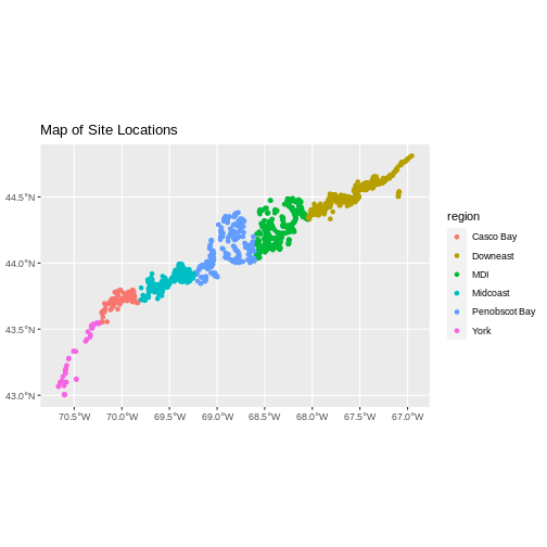
Looks good! If we really want to check, we can either load up our
state of Maine shapefile or plot it against a tiles with
leaflet.
R
library(leaflet)

pal <- colorFactor("Set1",
                   domain = dmr_sf$region)

leaflet() |>
  addTiles() |>
  addCircles(data = dmr_sf,
             color = ~pal(region))
R
# Load Casco
casco_dmr <- read.csv(
  "data/maine_dmr/casco_kelp_urchin.csv"
)


# Turn it into an sf object
casco_dmr_sf <- st_as_sf(casco_dmr,
                         coords = c("longitude", "latitude"),
                         crs = 4326)

# Load Maine
maine <- st_read(
  "data/maine_gov_maps/Maine_State_Boundary_Polygon_Feature/Maine_State_Boundary_Polygon_Feature.shp",
  quiet = TRUE)

# Crop to Casco
casco <- st_crop(maine |> st_make_valid(),
                 casco_dmr_sf)

# Plot!
ggplot() +
  geom_sf(data = casco) +
  geom_sf(data = casco_dmr_sf, color = "red")
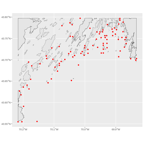
Key Points
Sometimes, we want to crop to a larger area than just the data set.
For that, we can create a box from the extent of the new vector object
using st_bbox(). This, though, is really just a vector, so
we need to turn it into a polygon using st_sfc() (sfc
objects are just a raw shape, while sf contains data).
To make this box bigger, we can use st_buffer() which
will create a buffer area using a distance specified in meters. So,
1e4 would be 10km.
This technique can be a nice way to put a new vector file in context, as follows.
R
#Make a bounding box of the Casco Bay area from the data
casco_bbox <- st_bbox(casco_dmr_sf) |>
  st_as_sfc()

# Enlarge it by 10 km
casco_bbox_big <- st_buffer(casco_bbox,
                            dist = 1e4)

# Crop to the new area
casco <- st_crop(maine |> st_make_valid(),
                 casco_bbox_big)

# Plot!
ggplot() +
  geom_sf(data = casco, fill = "darkgrey") +
  geom_sf(data = casco_dmr_sf, color = "red")
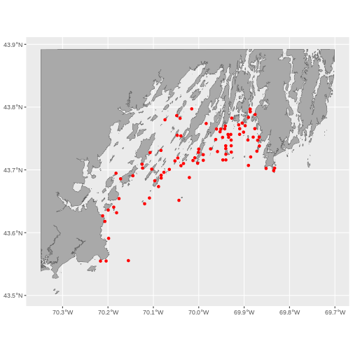
Export to an ESRI shapefile
We can write an R spatial object to an ESRI shapefile
using the st_write function in sf. To do this
we need the following arguments:
- the name of the spatial object (
dmr_sf) - the directory where we want to save our ESRI
shapefile(to usecurrent = getwd()or you can specify a different path). You can also usedir.create()no make a new directory. - the name of the new ESRI
shapefile(dmr_kelp_urchins) - the driver which specifies the file format (ESRI Shapefile)
We can now export the spatial object as an ESRI
shapefile. Note - this will make a few files.
R
dir.create("data/dmr_kelp_urchins")
st_write(dmr_sf,
         "data/dmr_kelp_urchins/dmr_kelp_urchins.shp", driver = "ESRI Shapefile")
Content from Extracting Data from Rasters using Vectors
Last updated on 2024-03-12 | Edit this page
Estimated time: 60 minutes
WARNING
Warning in
download.file("https://www.naturalearthdata.com/http//www.naturalearthdata.com/download/110m/physical/ne_110m_graticules_all.zip",
: cannot open URL
'https://www.naturalearthdata.com/http//www.naturalearthdata.com/download/110m/physical/ne_110m_graticules_all.zip':
HTTP status was '500 Internal Server Error'
ERROR
Error in download.file("https://www.naturalearthdata.com/http//www.naturalearthdata.com/download/110m/physical/ne_110m_graticules_all.zip", : cannot open URL 'https://www.naturalearthdata.com/http//www.naturalearthdata.com/download/110m/physical/ne_110m_graticules_all.zip'Overview
Questions
- How can I crop raster objects to vector objects, and extract the summary of raster pixels?
Objectives
- Crop a raster to the extent of a vector layer.
- Extract values from a raster that correspond to a vector file overlay.
Things You’ll Need To Complete This Episode
See the lesson homepage for detailed information about the software, data, and other prerequisites you will need to work through the examples in this episode.
Load Libraries
This episode explains how to crop a raster using the extent of a vector layer. We will also cover how to extract values from a raster that occur within a set of polygons, or in a buffer (surrounding) region around a set of points.
R
library(sf)
library(terra)
library(ggplot2)
library(tidyterra)
Crop a Raster to Vector Extent
We often work with spatial layers that have different spatial extents. The spatial extent of a vector layer or R spatial object represents the geographic “edge” or location that is the furthest north, south east and west. Thus it represents the overall geographic coverage of the spatial object.
 Image Source: National Ecological
Observatory Network (NEON)
The graphic below illustrates the extent of several of the spatial layers that we have worked with in this workshop and one new one:
- Area of interest (AOI) – blue
- Seagrass Beds – purple
- Areas surveyed for kelp and urchins (marked with white dots)– black
- Water turbidity in GeoTIFF format – green
R
# Casco AOI
aoi_boundary_casco <- st_read(
  "data/maine_gov_maps/casco_aoi/casco_bay_aoi.shp")

# seagrass in 2022
seagrass_casco_2022 <- st_read(
  "data/maine_gov_seagrass/MaineDEP_Casco_Bay_Seagrass_2022/MaineDEP_Casco_Bay_Seagrass_2022.shp")

# subtidal samples
dmr_casco <-
  read.csv("data/maine_dmr/casco_kelp_urchin.csv") |>
  st_as_sf(coords = c("longitude", "latitude"), crs = 4326)

# turbidity from modis
turbidity_modis <- rast("data/modis/GIOVANNI-g4.timeAvgMap.MODISA_L3m_KD_Mo_4km_R2022_0_Kd_490.20230701-20230930.71W_42N_66W_45N.tif")
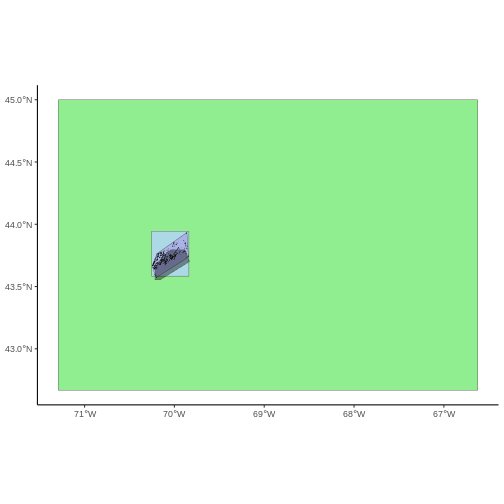
Frequent use cases of cropping a raster file include reducing file size and creating maps. Sometimes we have a raster file that is much larger than our study area or area of interest. It is often more efficient to crop the raster to the extent of our study area to reduce file sizes as we process our data. Cropping a raster can also be useful when creating pretty maps so that the raster layer matches the extent of the desired vector layers.
Crop a Raster Using Vector Extent
We can use the crop() function to crop a raster to the
extent of another spatial object. To do this, we need to specify the
raster to be cropped and the spatial object that will be used to crop
the raster. R will use the extent of the spatial object as
the cropping boundary.
To illustrate this, we will crop the MODIS turbidity data to only
include the area of interest (AOI). Let’s start by plotting the full
extent of the CHM data and overlay where the AOI falls within it. The
boundaries of the AOI will be colored blue, and we use
fill = NA to make the area transparent.
R
ggplot() +
  geom_spatraster(data = turbidity_modis) +
  scale_fill_gradientn(name = "Turbidity Score", colors = terrain.colors(10)) +
  geom_sf(data = aoi_boundary_casco, color = "blue", fill = NA) +
  coord_sf()
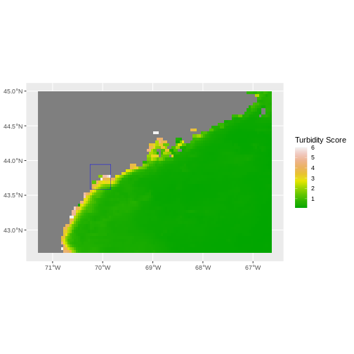
Now that we have visualized the area of the turbidity data we want to
subset, we can perform the cropping operation. We are going to
crop() function from the raster package to create a new
object with only the portion of the MODIS data that falls within the
boundaries of the AOI.
R
turbidity_casco <- crop(x = turbidity_modis, y = aoi_boundary_casco)
Now we can plot the cropped MODIS data, along with a boundary box
showing the full MODIS extent. However, remember, since this is raster
data, we need to convert to a data frame in order to plot using
ggplot. To get the boundary box from MODIS, the
st_bbox() will extract the 4 corners of the rectangle that
encompass all the features contained in this object. The
st_as_sfc() converts these 4 coordinates into a polygon
that we can plot:
R
ggplot() +
  geom_sf(data = st_as_sfc(st_bbox(turbidity_modis)), fill = "green",
          color = "green", alpha = .2) +
  geom_spatraster(data = turbidity_casco) +
  scale_fill_gradientn(name = "Turbidity Score", colors = terrain.colors(10)) +
  coord_sf()
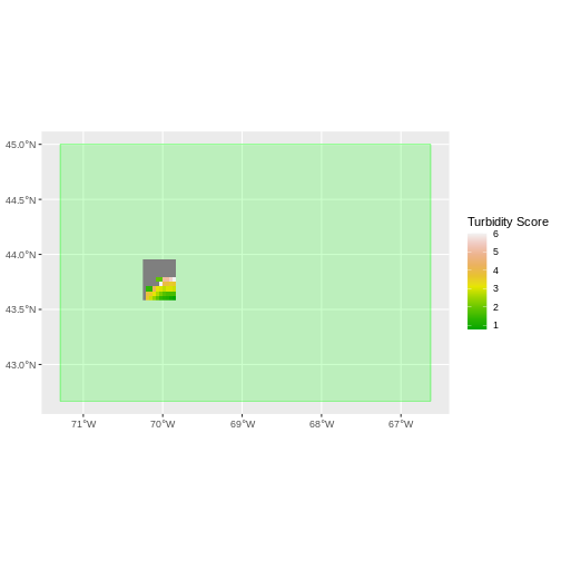
The plot above shows that the full MODS extent (plotted in green) is
much larger than the resulting cropped raster. Our new cropped MODS now
has the same extent as the aoi_boundary_casco object that
was used as a crop extent (blue border below).
R
ggplot() +
  geom_spatraster(data = turbidity_casco) +
  geom_sf(data = aoi_boundary_casco, color = "blue", fill = NA) +
  scale_fill_gradientn(name = "Turbidity Score", colors = terrain.colors(10)) +
  coord_sf()
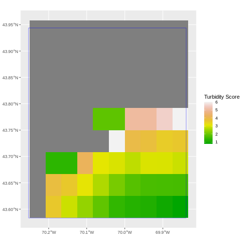
We can look at the extent of all of our other objects for this field site.
R
st_bbox(turbidity_modis)
OUTPUT
     xmin      ymin      xmax      ymax
-71.29166  42.66666 -66.62500  45.00000
R
st_bbox(turbidity_casco)
OUTPUT
     xmin      ymin      xmax      ymax
-70.25000  43.58333 -69.83333  43.95833
R
st_bbox(aoi_boundary_casco)
OUTPUT
    xmin     ymin     xmax     ymax
-70.2528  43.5834 -69.8387  43.9439
R
st_bbox(seagrass_casco_2022)
OUTPUT
     xmin      ymin      xmax      ymax
-70.24464  43.57213 -69.84399  43.93221
R
st_bbox(dmr_casco)
OUTPUT
     xmin      ymin      xmax      ymax
-70.21650  43.55470 -69.83280  43.79721
Our dmr_casco location extent is not the largest It
would be nice to see our vegetation plot locations plotted on top of the
turbidity information.
R
turbidity_dmr_sites <- crop(x = turbidity_modis, y = dmr_casco)

ggplot() +
  geom_spatraster(data = turbidity_dmr_sites) +
  scale_fill_gradientn(name = "Canopy Height", colors = terrain.colors(10)) +
  geom_sf(data = dmr_casco)
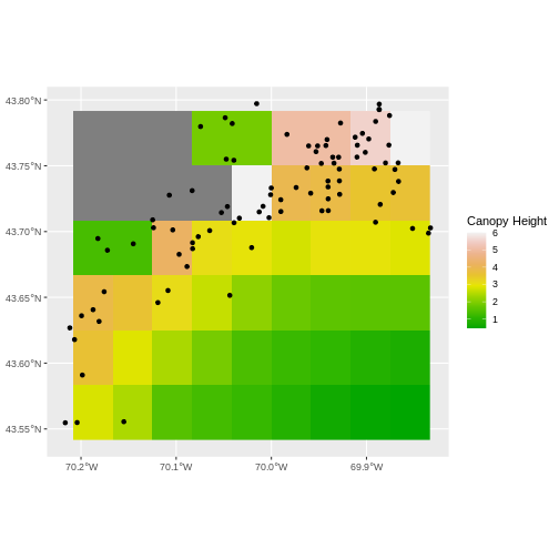
In the plot above, created in the challenge, all the site locations (black dots) appear on the turbidity raster layer except for a few. some are situated on the blank space to the left of the map. Why?
The raster data is in a resolution such that many of the coastal pixels are eliminated as not valid data. Check the resolution of the raster. It’s 0.417 degrees. 1 degree is ~ 111,111 meters. So, 1 pixel here is ~ 4,600 meters, or 4.6km. We are going to lose a lot of things close to the coast.
Thinking about data source resolution is key in thinking about rasters when you want to get data close to the coast versus more offshore.
Extract Raster Pixels Values Using Vector Polygons
Often we want to extract values from a raster layer for particular locations - for example, plot locations that we are sampling on the ground. We can extract all pixel values within 20m of our x,y point of interest. These can then be summarized into some value of interest (e.g. mean, maximum, total).
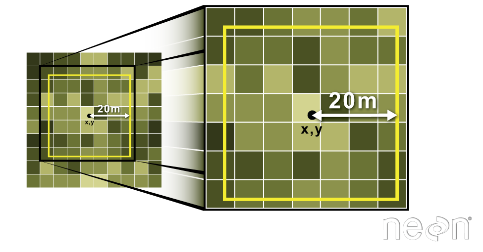 Image Source: National Ecological Observatory Network (NEON)
To do this in R, we use the extract() function. The
extract() function requires:
- The raster that we wish to extract values from,
- The vector layer containing the polygons that we wish to use as a boundary or boundaries,
- we can tell it to store the output values in a data frame using
raw = FALSE(this is optional).
We will begin by extracting all canopy height pixel values located
within our aoi_boundary_casco polygon which surrounds the
tower located at the NEON Harvard Forest field site.
R
names(turbidity_casco) <- "turbidity"

turbidity_df <- extract(x = turbidity_casco,
                     y = aoi_boundary_casco,
                     raw = FALSE)

str(turbidity_df)
OUTPUT
'data.frame':	90 obs. of  2 variables:
 $ ID       : num  1 1 1 1 1 1 1 1 1 1 ...
 $ turbidity: num  NA NA NA NA NA NA NA NA NA NA ...
When we use the extract() function, R extracts the value
for each pixel located within the boundary of the polygon being used to
perform the extraction - in this case the
aoi_boundary_casco object (a single polygon). Here, the
function extracted values from 90 pixels.
We can create a histogram of turbidity values within the boundary to
better understand the structure or height distribution of turbidity at
our site. We will use the column turbidity from our data
frame as our x values.
R
ggplot() +
  geom_histogram(data = turbidity_df, aes(x = turbidity)) +
  ggtitle("Histogram of turbidity values") +
  xlab("turbidity") +
  ylab("Frequency of Pixels")
OUTPUT
`stat_bin()` using `bins = 30`. Pick better value with `binwidth`.WARNING
Warning: Removed 52 rows containing non-finite values (`stat_bin()`).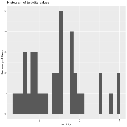
We can also use the summary() function to view
descriptive statistics including min, max, and mean height values. These
values help us better understand vegetation at our field site.
R
summary(turbidity_df$turbidity)
OUTPUT
   Min. 1st Qu.  Median    Mean 3rd Qu.    Max.    NA's
 0.7771  1.6590  2.8625  2.8668  3.6165  6.0000      52
Summarize Extracted Raster Values
We often want to extract summary values from a raster. We can tell R
the type of summary statistic we are interested in using the
fun = argument. Let’s extract a mean height value for our
AOI.
R
mean_turbidity_aoi <- extract(x = turbidity_casco,
                                 y = aoi_boundary_casco,
                                fun = mean, na.rm = TRUE)

mean_turbidity_aoi
OUTPUT
  ID turbidity
1  1  2.866811
It appears that the mean height value, extracted from our LiDAR data derived canopy height model is 22.43 meters.
Extract Data using x,y Locations
We can also extract pixel values from a raster by defining a buffer
or area surrounding individual point locations using the
st_buffer() function. To do this we define the summary
argument (fun = mean) and the buffer distance
(dist = 20) which represents the radius of a circular
region around each point. By default, the units of the buffer are the
same units as the data’s CRS. All pixels that are touched by the buffer
region are included in the extract.
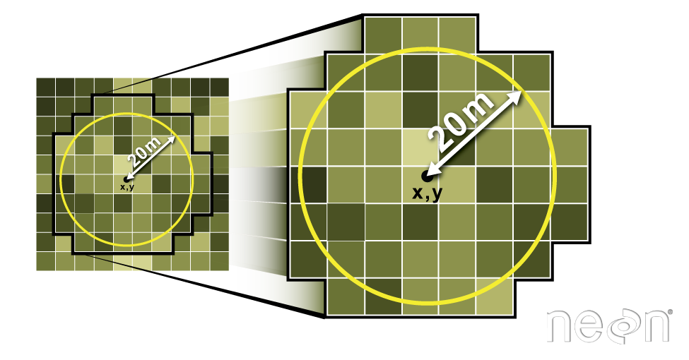 Image Source: National Ecological Observatory Network (NEON)
Let’s put this into practice by figuring out the mean tree height in
the 20m around the tower location (point_HARV).
R
mean_turbidity_sites <- extract(x = turbidity_casco,
                                  y = st_buffer(dmr_casco, dist = 20),
                                  fun = mean,
                                raw = FALSE)

hist(mean_turbidity_sites$turbidity)
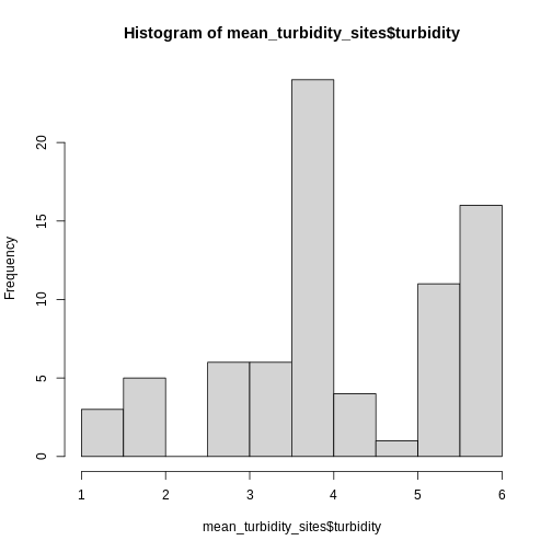
Challenge: Extract Temperature Values For Seagrass Beds
You can also extract data from polygons. Let’s look at temperature in seagrass beds in 2022.
Load up “data/landsat_casco/b10_cropped/LC08_L2SP_011030_20220909_20220914_02_T1_ST_B10.TIF”. Reproject it and crop it to the extent of
seagrass_casco_2022- smaller rasters = faster extraction.Extract the average SST in each bed.
cbind()it back toseagrass_casco_2022Plot SST by Hectares of seagrass bed.
- We can do this as a processing chain!
R
sst <- rast(
  "data/landsat_casco/b10_cropped/LC08_L2SP_011030_20220909_20220914_02_T1_ST_B10.TIF"
  ) |>
  project(crs(seagrass_casco_2022)) |>
  crop(seagrass_casco_2022)
- We can extract now. Note, some beds will throw an NaN, as
R
temp_beds <- extract(sst,
                     seagrass_casco_2022,
                     fun = mean,
                     na.rm = TRUE,
                     raw = FALSE)

seagrass_casco_2022 <- cbind(seagrass_casco_2022, temp_beds)
- It’s just a
geom_point()
R
ggplot(data = seagrass_casco_2022) +
  geom_point(aes(x = SST_F_20220909, y = Hectares))
WARNING
Warning: Removed 314 rows containing missing values (`geom_point()`).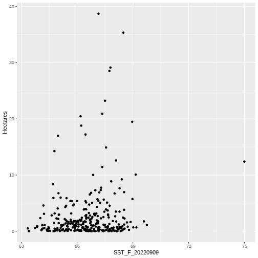
Content from Work with Multi-Band Rasters
Last updated on 2024-03-12 | Edit this page
Estimated time: 60 minutes
WARNING
Warning in
download.file("https://www.naturalearthdata.com/http//www.naturalearthdata.com/download/110m/physical/ne_110m_graticules_all.zip",
: cannot open URL
'https://www.naturalearthdata.com/http//www.naturalearthdata.com/download/110m/physical/ne_110m_graticules_all.zip':
HTTP status was '500 Internal Server Error'
ERROR
Error in download.file("https://www.naturalearthdata.com/http//www.naturalearthdata.com/download/110m/physical/ne_110m_graticules_all.zip", : cannot open URL 'https://www.naturalearthdata.com/http//www.naturalearthdata.com/download/110m/physical/ne_110m_graticules_all.zip'Overview
Questions
- How can I visualize individual and multiple bands in a raster object?
Objectives
- Identify a single vs. a multi-band raster file.
- Import multi-band rasters into R using the
terrapackage. - Plot multi-band color image rasters in R using the
ggplotpackage.
First, some libraries you might not have loaded at the moment.
R
library(terra)
library(ggplot2)
library(dplyr)
library(tidyterra)
Things You’ll Need To Complete This Episode
See the lesson homepage for detailed information about the software, data, and other prerequisites you will need to work through the examples in this episode.
We introduced multi-band raster data in an earlier lesson. This episode explores how to import and plot a multi-band raster in R.
Getting Started with Multi-Band Data in R
In this episode, the multi-band data that we are working with is imagery collected using the Landsat 8 Satellite satellite on row 12 path 30 of it’s traverse around the planet. Landsat is a series of multispectral satellites with a 30m pixel resolution. This means that each image has multiple wavelengths of light observed - not just Red, Green, and Blue (RGB). Here are the bands of the Landsat 8 OLI:
- Band 1 Coastal Aerosol (0.43 - 0.45 µm) 30 m
- Band 2 Blue (0.450 - 0.51 µm) 30 m
- Band 3 Green (0.53 - 0.59 µm) 30 m
- Band 4 Red (0.64 - 0.67 µm) 30 m
- Band 5 Near-Infrared (0.85 - 0.88 µm) 30 m
- Band 6 SWIR 1(1.57 - 1.65 µm) 30 m
- Band 7 SWIR 2 (2.11 - 2.29 µm) 30 m
- Band 8 Panchromatic (PAN) (0.50 - 0.68 µm) 15 m
- Band 9 Cirrus (1.36 - 1.38 µm) 30 m
So, 4, 3, and 2 are RGB. By using the rast() function we
can read one raster bands (i.e. the first one) or many.
Let’s start by looking at the red band.
R
landsat_band4_1230 <-
  rast("data/landsat_casco/LC08_L2SP_012030_20230903_20230912_02_T1/LC08_L2SP_012030_20230903_20230912_02_T1_SR_B4.TIF")

ggplot() +
  geom_spatraster(data = landsat_band4_1230) +
  scale_fill_distiller(palette = "Greys")
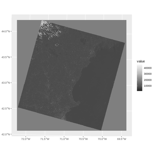
R
landsat_band4_1230
OUTPUT
class       : SpatRaster
dimensions  : 7991, 7891, 1  (nrow, ncol, nlyr)
resolution  : 30, 30  (x, y)
extent      : 232485, 469215, 4662585, 4902315  (xmin, xmax, ymin, ymax)
coord. ref. : WGS 84 / UTM zone 19N (EPSG:32619)
source      : LC08_L2SP_012030_20230903_20230912_02_T1_SR_B4.TIF
name        : LC08_L2SP_012030_20230903_20230912_02_T1_SR_B4
Notice that when we look at the attributes of this band, we see:
dimensions : 7991, 7891, 1 (nrow, ncol, nlyr)
This is R telling us that we read only one band.
Raster Stacks in R
Next, we will work with mutiple bands as an R raster object. We will then plot a 3-band composite, or full color, image, and what is called a ‘fasle-color’ image.
To bring in all bands of a multi-band raster, we use
therast() function.
For multi-layer views, we need to look at all of the files we get with a typical sensor image. They are often listed as different files (although they can come in one big file.) Let’s see what a typical Landsat image has.
R
list.files("data/landsat_casco/LC08_L2SP_012030_20230903_20230912_02_T1/")
OUTPUT
 [1] "LC08_L2SP_012030_20230903_20230912_02_T1_ANG.txt"
 [2] "LC08_L2SP_012030_20230903_20230912_02_T1_MTL.txt"
 [3] "LC08_L2SP_012030_20230903_20230912_02_T1_MTL.xml"
 [4] "LC08_L2SP_012030_20230903_20230912_02_T1_QA_PIXEL.TIF"
 [5] "LC08_L2SP_012030_20230903_20230912_02_T1_QA_RADSAT.TIF"
 [6] "LC08_L2SP_012030_20230903_20230912_02_T1_SR_B1.TIF"
 [7] "LC08_L2SP_012030_20230903_20230912_02_T1_SR_B2.TIF"
 [8] "LC08_L2SP_012030_20230903_20230912_02_T1_SR_B3.TIF"
 [9] "LC08_L2SP_012030_20230903_20230912_02_T1_SR_B4.TIF"
[10] "LC08_L2SP_012030_20230903_20230912_02_T1_SR_B5.TIF"
[11] "LC08_L2SP_012030_20230903_20230912_02_T1_SR_B6.TIF"
[12] "LC08_L2SP_012030_20230903_20230912_02_T1_SR_B7.TIF"
[13] "LC08_L2SP_012030_20230903_20230912_02_T1_SR_QA_AEROSOL.TIF"
That’s a lot of files! To load them in with rast() in a
single object, thought, we will want only those that are TIF files, and
we will need the full path to each one. Fortunately,
list.files() makes that easy for us.
R
landsat_files <-
  list.files("data/landsat_casco/LC08_L2SP_012030_20230903_20230912_02_T1",
             full.names = TRUE,
             pattern = "TIF")

landsat_files
OUTPUT
 [1] "data/landsat_casco/LC08_L2SP_012030_20230903_20230912_02_T1/LC08_L2SP_012030_20230903_20230912_02_T1_QA_PIXEL.TIF"
 [2] "data/landsat_casco/LC08_L2SP_012030_20230903_20230912_02_T1/LC08_L2SP_012030_20230903_20230912_02_T1_QA_RADSAT.TIF"
 [3] "data/landsat_casco/LC08_L2SP_012030_20230903_20230912_02_T1/LC08_L2SP_012030_20230903_20230912_02_T1_SR_B1.TIF"
 [4] "data/landsat_casco/LC08_L2SP_012030_20230903_20230912_02_T1/LC08_L2SP_012030_20230903_20230912_02_T1_SR_B2.TIF"
 [5] "data/landsat_casco/LC08_L2SP_012030_20230903_20230912_02_T1/LC08_L2SP_012030_20230903_20230912_02_T1_SR_B3.TIF"
 [6] "data/landsat_casco/LC08_L2SP_012030_20230903_20230912_02_T1/LC08_L2SP_012030_20230903_20230912_02_T1_SR_B4.TIF"
 [7] "data/landsat_casco/LC08_L2SP_012030_20230903_20230912_02_T1/LC08_L2SP_012030_20230903_20230912_02_T1_SR_B5.TIF"
 [8] "data/landsat_casco/LC08_L2SP_012030_20230903_20230912_02_T1/LC08_L2SP_012030_20230903_20230912_02_T1_SR_B6.TIF"
 [9] "data/landsat_casco/LC08_L2SP_012030_20230903_20230912_02_T1/LC08_L2SP_012030_20230903_20230912_02_T1_SR_B7.TIF"
[10] "data/landsat_casco/LC08_L2SP_012030_20230903_20230912_02_T1/LC08_L2SP_012030_20230903_20230912_02_T1_SR_QA_AEROSOL.TIF"
Great! We can now load those in smoothly with
rast().
R
# load all bands
landsat_all_1230 <- rast(landsat_files)

landsat_all_1230
OUTPUT
class       : SpatRaster
dimensions  : 7991, 7891, 10  (nrow, ncol, nlyr)
resolution  : 30, 30  (x, y)
extent      : 232485, 469215, 4662585, 4902315  (xmin, xmax, ymin, ymax)
coord. ref. : WGS 84 / UTM zone 19N (EPSG:32619)
sources     : LC08_L2SP_012030_20230903_20230912_02_T1_QA_PIXEL.TIF
              LC08_L2SP_012030_20230903_20230912_02_T1_QA_RADSAT.TIF
              LC08_L2SP_012030_20230903_20230912_02_T1_SR_B1.TIF
              ... and 7 more source(s)
names       : LC08_~PIXEL, LC08_~ADSAT, LC08_~SR_B1, LC08_~SR_B2, LC08_~SR_B3, LC08_~SR_B4, ...
Now we have a very different set of dimensions and names.
dimensions : 7991, 7891, 10 (nrow, ncol, nlyr)
10 bands! To see what is loaded, we can just use
names()
R
names(landsat_all_1230)
OUTPUT
 [1] "LC08_L2SP_012030_20230903_20230912_02_T1_QA_PIXEL"
 [2] "LC08_L2SP_012030_20230903_20230912_02_T1_QA_RADSAT"
 [3] "LC08_L2SP_012030_20230903_20230912_02_T1_SR_B1"
 [4] "LC08_L2SP_012030_20230903_20230912_02_T1_SR_B2"
 [5] "LC08_L2SP_012030_20230903_20230912_02_T1_SR_B3"
 [6] "LC08_L2SP_012030_20230903_20230912_02_T1_SR_B4"
 [7] "LC08_L2SP_012030_20230903_20230912_02_T1_SR_B5"
 [8] "LC08_L2SP_012030_20230903_20230912_02_T1_SR_B6"
 [9] "LC08_L2SP_012030_20230903_20230912_02_T1_SR_B7"
[10] "LC08_L2SP_012030_20230903_20230912_02_T1_SR_QA_AEROSOL"We just want red, green, blue, and near-infrared for now - bands 2 through 5. Note how that corresponds to layers 4 through 7. So we can subset down.
R
landsat_colors_1230 <- subset(landsat_all_1230,
                              subset = 4:7)
Let’s preview the attributes of our stack object:
R
landsat_colors_1230
OUTPUT
class       : SpatRaster
dimensions  : 7991, 7891, 4  (nrow, ncol, nlyr)
resolution  : 30, 30  (x, y)
extent      : 232485, 469215, 4662585, 4902315  (xmin, xmax, ymin, ymax)
coord. ref. : WGS 84 / UTM zone 19N (EPSG:32619)
sources     : LC08_L2SP_012030_20230903_20230912_02_T1_SR_B2.TIF
              LC08_L2SP_012030_20230903_20230912_02_T1_SR_B3.TIF
              LC08_L2SP_012030_20230903_20230912_02_T1_SR_B4.TIF
              LC08_L2SP_012030_20230903_20230912_02_T1_SR_B5.TIF
names       : LC08_L2~1_SR_B2, LC08_L2~1_SR_B3, LC08_L2~1_SR_B4, LC08_L2~1_SR_B5
We can view the attributes of each band in the stack in a single output. For example, if we had hundreds of bands, we could specify which band we’d like to view attributes for using an index value:
R
landsat_colors_1230[[2]]
OUTPUT
class       : SpatRaster
dimensions  : 7991, 7891, 1  (nrow, ncol, nlyr)
resolution  : 30, 30  (x, y)
extent      : 232485, 469215, 4662585, 4902315  (xmin, xmax, ymin, ymax)
coord. ref. : WGS 84 / UTM zone 19N (EPSG:32619)
source      : LC08_L2SP_012030_20230903_20230912_02_T1_SR_B3.TIF
name        : LC08_L2SP_012030_20230903_20230912_02_T1_SR_B3
We can also use the ggplot functions to plota histogram
of the first (blue) band:
R
ggplot() +
  geom_histogram(data = landsat_colors_1230,
                 aes(x = LC08_L2SP_012030_20230903_20230912_02_T1_SR_B3),
                 bins = 1e4)
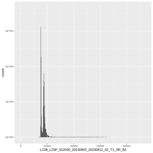
This tells us that, for example, we might want to cutoff high quantiles when we start to blend colors for an RGB plot.
We can also plot all of the bands with either
plot() or ggplot() adding a
facet_wrap(facets = vars(lyr)) call to facet by layer.
R
#plot(landsat_colors_1230)

ggplot() +
  geom_spatraster(data = landsat_colors_1230) +
  facet_wrap(facets = vars(lyr)) +
  scale_fill_distiller(palette = "Greys")
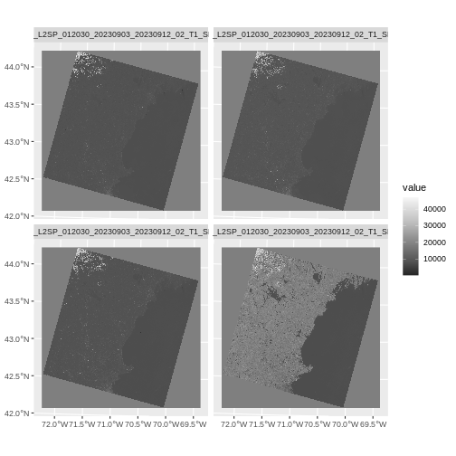
R
ggplot() +
  geom_spatraster(data = landsat_colors_1230[[3:4]]) +
  facet_wrap(facets = vars(lyr)) +
  scale_fill_viridis_b()
We’d expect a brighter value for the land in band 5 (NIR) than in band 4 (red) because healthy vegetation reflects MORE NIR light than red light.
Create A Three Band Image
To render a final three band, colored image in R, we use the
plotRGB() or geom_spatraster_rgb()
function.
This function allows us to:
Identify what bands we want to render in the red, green and blue regions. The
plotRGB()function defaults to a 1=red, 2=green, and 3=blue band order. However, you can define what bands you’d like to plot manually. Manual definition of bands is useful if you have, for example a near-infrared band and want to create a color infrared image.Adjust the
stretchof the image to increase or decrease contrast.
Let’s plot our 3-band image. Note that we can use the
plotRGB() function directly with our RasterStack object (we
don’t need a dataframe as this function isn’t part of the
ggplot2 package).
R
plotRGB(landsat_colors_1230,
        r = 3, g = 2, b = 1)
That throws an error as sometimes plotRGB doesn’t like really large values when it rescales. RGB values for a computer screen are typically between 0 and 255, so, we just need to rescale our values between 0 and 255. We can do that by multiplying the raster values by 255/(max of the raster values). Note, you can either do this so EACH channel is rescalled to 0-255, or, they are all rescaled by one grand value.
R
colmax <- max(landsat_colors_1230[[1:3]]) |> values() |> max(na.rm = TRUE)

colmax

plotRGB(landsat_colors_1230 * 255/colmax,
        r = 3, g = 2, b = 1, main = "Rescaled for each channel")
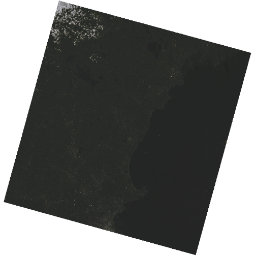
The image above looks OK, but dark. You can actually play with the
denominator of the scaling to make more interesting ones, or scale by
other rasters. But, there are more standard (and better) stretching
algorithms. We can explore whether applying a stretch to the image might
improve clarity and contrast using stretch="lin" or
stretch="hist".
When the range of pixel brightness values is closer to 0, a darker image is rendered by default. We can stretch the values to extend to the full 0-255 range of potential values to increase the visual contrast of the image.
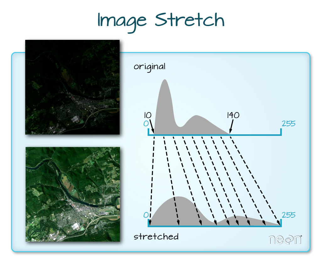
When the range of pixel brightness values is closer to 255, a lighter image is rendered by default. We can stretch the values to extend to the full 0-255 range of potential values to increase the visual contrast of the image.
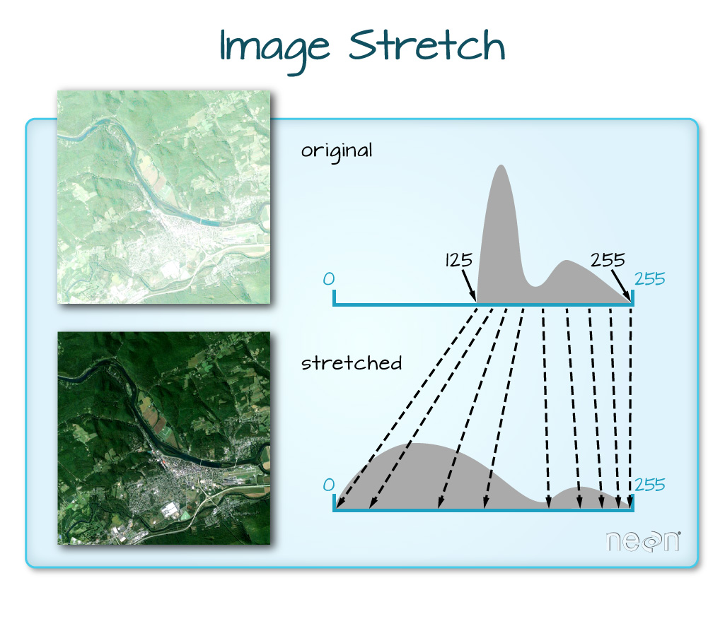
We can implement this easily in R where we not only make a linear stretch, but chop off some of the highest and lowest values.
R
plotRGB(landsat_colors_1230,
        r = 1, g = 2, b = 3,
        stretch = "lin")
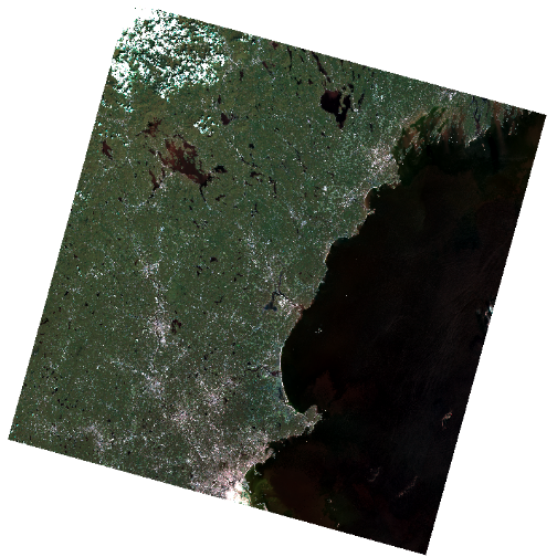
If the problem is that we want an even distribution of values for
each channel, rather than clumps and clusters, we use hist
as our stretch.
R
plotRGB(landsat_colors_1230,
        r = 1, g = 2, b = 3,
        stretch = "hist")
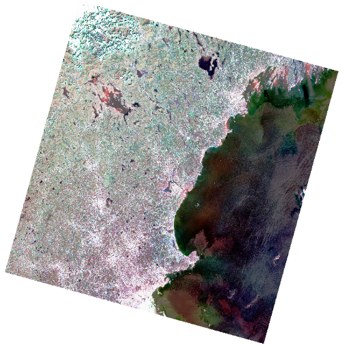
In this case, the stretch begins to show some things happening offshore a bit more, which might prompt more investigation.
Note, to do this with ggplot2, we need to apply
stretch() to the raster first and cut off the lower and
upper quantile of values. We can then use
geom_spatraster_rgb(). Note, to use stretch()
and get the RGB right, we need to reference the layer numbers of the
raster as indices.
R
ggplot() +
  geom_spatraster_rgb(data = stretch(landsat_colors_1230[[c(3,2,1)]],
                                 minq = 0.02, maxq = 0.98))
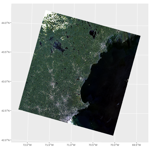
Challenge - False Color Images
What we have plotted above is a True Color Image. To help see things, many people use False color Images. Either they switch the bands (so, GRB instead of RGB) or use other bands. What do you see that is different if you try the following. Apply any stretch you like.
- Instead of RGB, plot GRB.
- Instead of RBG, plot NRG (where N = NIR). This creates a ‘vegetation in red’ map, which can be useful for vegetation.
- Note how we use r, g, and b as channel 1, 2, and 3.
R
plotRGB(landsat_colors_1230,
        r = 2, g = 3, b = 1,
        stretch = "lin")
- Here if you stretch with hist,you can get a better split between very vegetated and urbanized areas.
R
plotRGB(landsat_colors_1230,
        r = 4, g = 3, b = 2,
        stretch = "hist")
Data Tip
You can create interactive RGB overlays as well. But it takes some
extra doing, as you have to downsample large images, as
geom_spatraster() does natively. You can do this with
spatSample(). leaflet currently does odd
things to RGB rasters, so, you should use the leafem
library. Which does not yet handle SpatRaster objects from
terra. Fortunately, it’s a small thing to convert it to an
old school raster stack with raster::stack()
(we’re not loading the whole library to prevent conflicts in function
names). Note, for big rasters, you can up maxbytes in the
addRasterRGB from it’s default of 4*1024*1024,
but, this can cause plotting to take a very very very long time.
R
library(leaflet)
library(leafem)

# resample and then convert to a raster::stack object
# note, if this raster was small, we wouldn't have to
# spatSample()
landsat_colors_raster <- landsat_colors_1230 |>
  spatSample(size = 5e5, as.raster = TRUE, method = "regular")|>
  raster::stack()

# plot using addRasterRGB from leafem
leaflet() |>
  addRasterRGB(x = landsat_colors_raster,
               quantiles = c(0.02, 0.98))
Content from Raster Calculations
Last updated on 2024-03-12 | Edit this page
Estimated time: 60 minutes
ERROR
Error in download.file("https://www.naturalearthdata.com/http//www.naturalearthdata.com/download/110m/physical/ne_110m_graticules_all.zip", : cannot open URL 'https://www.naturalearthdata.com/http//www.naturalearthdata.com/download/110m/physical/ne_110m_graticules_all.zip'Overview
Questions
- How do I do math on rasters and extract pixel values for defined locations?
Objectives
- Perform a math with different raster layers.
- Perform more math using the raster
lapp()function. - Export raster data as a GeoTIFF file.
Things You’ll Need To Complete This Episode
See the lesson homepage for detailed information about the software, data, and other prerequisites you will need to work through the examples in this episode.
You will also need some new data that
you should unzip and put into the data/landsat_casco
folder.
We often want to combine values of and perform calculations on
rasters to create a new output raster. This episode covers how to
subtract one raster from another using basic raster math and the
lapp() function. It also covers how to extract pixel values
from a set of locations - for example a buffer region around plot
locations at a field site.
Raster Calculations in R
We often want to perform calculations on two or more rasters to create a new output raster. For example, if we are interested in getting the observed chlorophyll in the water, we might want to use different Landsat layers to calculate an observed value based on published equations. This can help us identify Suberged Aquatic Vegetation (SAV). The resulting data set might show us where seagrass or other vegetation exists. There are two method for this we will use today from Zhang 2023 and O’Reilly and Werdell in 2019. The first is a calculation of chlorophyll based on three bands that cover different nm of the visible spectrum.

Recall from before that the first few bands of Landsat 8 cover the following: - Band 1 Coastal Aerosol (430 - 450 nm) 30 m - Band 2 Blue (450 - 510 nm) 30 m - Band 3 Green (530 - 590 nm) 30 m - Band 4 Red (640 - 670 nm) 30 m - Band 5 Near-Infrared (850 - 880 nm) 30 m
To calculate Chla in the water, we will use imagery from Landsat that has been algorithmically corrected for water - i.e., algorithms that don’t just correct the imagery for things in the atmosphere, but that literally try their best to correct for all of the spectral properties of what is in the water. We are going to use three bands from a Landsat scene in winter of 2023, as phytoplankton is at a low and we are more likely to see what is on the seafloor. The imagery has been corrected using ACOLITE. With the three bands, in units of Rrs - in essence water leaving irradiance / downwellign irradiance. To learn more, see here.
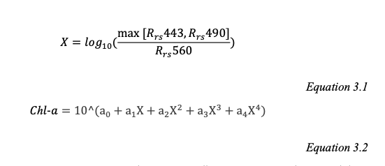
Where those a coefficients come from NASA Algorithms. Those three wavelengths correspond to the coastal band, the green band, and the blue band.
The second method is a bit simpler. It’s called the Chlorophyll Absorption Ratio Index (CARI).
 Let’s see how simple it is
to make these work for us!
More Resources
Chlorophyll A algorithms and NASA Earthdata.
O’Reilly, J. E., & Werdell, P. J. (2019). Chlorophyll algorithms for ocean color sensors-OC4, OC5 & OC6. https://doi.org/10.1016/j.rse.2019.04.021
Load Libraries and Pre-Process the Data

For this episode, we will use the Landsat scene from 2023 and the
seagrass beds from Casco Bay in 2022 (we’ll assume they’re close enough
to 2023). Let’s start by loading terra, sf,
and ggplot2.
R
library(terra)
library(sf)
library(ggplot2)
library(tidyterra)
Next, let’s load our two different data sources. We will load the rasters into one stack for ease of use. We will also load the Casco AOI and Maine State borders for use in cropping and masking down to just water.
R
# ACOLITE corrected Rrs - note, just the tifs, as the png is a thumbnail
landsat_files <- list.files(
  "data/landsat_casco/L8_OLI_2023_02_07_15_27_04_012030_L2R/",
           pattern = "tif",
           full.names = TRUE)

# Load all of the tifs
landsat_layers <- rast(landsat_files)

# give the layers better names
names(landsat_layers) <- c("blue_443", "blue_483", "green_561")

# load our shapefile
seagrass_casco_2022 <- st_read(
  "data/maine_gov_seagrass/MaineDEP_Casco_Bay_Seagrass_2022/MaineDEP_Casco_Bay_Seagrass_2022.shp")

# Load files for processing
aoi_boundary_casco <- st_read(
  "data/maine_gov_maps/casco_aoi/casco_bay_aoi.shp")

maine_borders <- st_read(
  "data/maine_gov_maps/Maine_State_Boundary_Polygon_Feature/Maine_State_Boundary_Polygon_Feature.shp")
R
describe(sources(landsat_layers))
OUTPUT
  [1] "Driver: GTiff/GeoTIFF"
  [2] "Files: /home/runner/work/r-raster-vector-geospatial/r-raster-vector-geospatial/site/built/data/landsat_casco/L8_OLI_2023_02_07_15_27_04_012030_L2R/L8_OLI_2023_02_07_15_27_04_012030_L2W_Rrs_443.tif"
  [3] "Size is 7891, 8001"
  [4] "Coordinate System is:"
  [5] "PROJCRS[\"WGS 84 / UTM zone 19N\","
  [6] "    BASEGEOGCRS[\"WGS 84\","
  [7] "        DATUM[\"World Geodetic System 1984\","
  [8] "            ELLIPSOID[\"WGS 84\",6378137,298.257223563,"
  [9] "                LENGTHUNIT[\"metre\",1]]],"
 [10] "        PRIMEM[\"Greenwich\",0,"
 [11] "            ANGLEUNIT[\"degree\",0.0174532925199433]],"
 [12] "        ID[\"EPSG\",4326]],"
 [13] "    CONVERSION[\"UTM zone 19N\","
 [14] "        METHOD[\"Transverse Mercator\","
 [15] "            ID[\"EPSG\",9807]],"
 [16] "        PARAMETER[\"Latitude of natural origin\",0,"
 [17] "            ANGLEUNIT[\"degree\",0.0174532925199433],"
 [18] "            ID[\"EPSG\",8801]],"
 [19] "        PARAMETER[\"Longitude of natural origin\",-69,"
 [20] "            ANGLEUNIT[\"degree\",0.0174532925199433],"
 [21] "            ID[\"EPSG\",8802]],"
 [22] "        PARAMETER[\"Scale factor at natural origin\",0.9996,"
 [23] "            SCALEUNIT[\"unity\",1],"
 [24] "            ID[\"EPSG\",8805]],"
 [25] "        PARAMETER[\"False easting\",500000,"
 [26] "            LENGTHUNIT[\"metre\",1],"
 [27] "            ID[\"EPSG\",8806]],"
 [28] "        PARAMETER[\"False northing\",0,"
 [29] "            LENGTHUNIT[\"metre\",1],"
 [30] "            ID[\"EPSG\",8807]]],"
 [31] "    CS[Cartesian,2],"
 [32] "        AXIS[\"(E)\",east,"
 [33] "            ORDER[1],"
 [34] "            LENGTHUNIT[\"metre\",1]],"
 [35] "        AXIS[\"(N)\",north,"
 [36] "            ORDER[2],"
 [37] "            LENGTHUNIT[\"metre\",1]],"
 [38] "    USAGE["
 [39] "        SCOPE[\"Engineering survey, topographic mapping.\"],"
 [40] "        AREA[\"Between 72°W and 66°W, northern hemisphere between equator and 84°N, onshore and offshore. Aruba. Bahamas. Brazil. Canada - New Brunswick (NB); Labrador; Nunavut; Nova Scotia (NS); Quebec. Colombia. Dominican Republic. Greenland. Netherlands Antilles. Puerto Rico. Turks and Caicos Islands. United States. Venezuela.\"],"
 [41] "        BBOX[0,-72,84,-66]],"
 [42] "    ID[\"EPSG\",32619]]"
 [43] "Data axis to CRS axis mapping: 1,2"
 [44] "Origin = (227370.000000000000000,4902630.000000000000000)"
 [45] "Pixel Size = (30.000000000000000,-30.000000000000000)"
 [46] "Metadata:"
 [47] "  AREA_OR_POINT=Area"
 [48] "  NC_GLOBAL#1_f0=19142.12138055756"
 [49] "  NC_GLOBAL#1_name=443"
 [50] "  NC_GLOBAL#1_wave=442.9823263713434"
 [51] "  NC_GLOBAL#2_f0=20166.79005236374"
 [52] "  NC_GLOBAL#2_name=483"
 [53] "  NC_GLOBAL#2_wave=482.5891954914198"
 [54] "  NC_GLOBAL#3_f0=18674.24059678011"
 [55] "  NC_GLOBAL#3_name=561"
 [56] "  NC_GLOBAL#3_wave=561.3326591091178"
 [57] "  NC_GLOBAL#4_f0=15649.95869773406"
 [58] "  NC_GLOBAL#4_name=655"
 [59] "  NC_GLOBAL#4_wave=654.606047604168"
 [60] "  NC_GLOBAL#5_f0=9484.951897185036"
 [61] "  NC_GLOBAL#5_name=865"
 [62] "  NC_GLOBAL#5_wave=864.5710906521408"
 [63] "  NC_GLOBAL#6_f0=2387.412329710507"
 [64] "  NC_GLOBAL#6_name=1609"
 [65] "  NC_GLOBAL#6_wave=1609.090443719705"
 [66] "  NC_GLOBAL#7_f0=814.198506038592"
 [67] "  NC_GLOBAL#7_name=2201"
 [68] "  NC_GLOBAL#7_wave=2201.248051984069"
 [69] "  NC_GLOBAL#8_f0=17580.89139262524"
 [70] "  NC_GLOBAL#8_name=592"
 [71] "  NC_GLOBAL#8_wave=591.6668530611159"
 [72] "  NC_GLOBAL#9_f0=3585.513285112"
 [73] "  NC_GLOBAL#9_name=1373"
 [74] "  NC_GLOBAL#9_wave=1373.476437717959"
 [75] "  NC_GLOBAL#acolite_file_type=L2R"
 [76] "  NC_GLOBAL#acolite_version=Generic GitHub Clone c2023-10-25T11:06:29"
 [77] "  NC_GLOBAL#acstar3_ex=3"
 [78] "  NC_GLOBAL#acstar3_fit_all_bands=True"
 [79] "  NC_GLOBAL#acstar3_mask_edges=True"
 [80] "  NC_GLOBAL#acstar3_max_wavelength=720"
 [81] "  NC_GLOBAL#acstar3_method=iter"
 [82] "  NC_GLOBAL#acstar3_psf_raster=False"
 [83] "  NC_GLOBAL#acstar3_write_rhoa=True"
 [84] "  NC_GLOBAL#acstar3_write_rhoe=True"
 [85] "  NC_GLOBAL#acstar3_write_rhosu=True"
 [86] "  NC_GLOBAL#add_band_name=False"
 [87] "  NC_GLOBAL#adjacency_correction=False"
 [88] "  NC_GLOBAL#adjacency_method=acstar3"
 [89] "  NC_GLOBAL#aerosol_correction=dark_spectrum"
 [90] "  NC_GLOBAL#ancillary_data=True"
 [91] "  NC_GLOBAL#ancillary_type=GMAO_MERRA2_MET"
 [92] "  NC_GLOBAL#atmospheric_correction=True"
 [93] "  NC_GLOBAL#auto_grouping=rhot:rhorc:rhos:rhow:Rrs:Lt"
 [94] "  NC_GLOBAL#blackfill_max=1.0"
 [95] "  NC_GLOBAL#blackfill_skip=True"
 [96] "  NC_GLOBAL#blackfill_wave=1600"
 [97] "  NC_GLOBAL#chris_interband_calibration=False"
 [98] "  NC_GLOBAL#chris_noise_reduction=True"
 [99] "  NC_GLOBAL#cirrus_correction=False"
[100] "  NC_GLOBAL#cirrus_g_swir=0.5"
[101] "  NC_GLOBAL#cirrus_g_vnir=1.0"
[102] "  NC_GLOBAL#cirrus_range={1350,1390}"
[103] "  NC_GLOBAL#clear_scratch=True"
[104] "  NC_GLOBAL#compute_contrabands=True"
[105] "  NC_GLOBAL#contact=Quinten Vanhellemont"
[106] "  NC_GLOBAL#Conventions=CF-1.7"
[107] "  NC_GLOBAL#copy_datasets={lon,lat,sza,vza,raa,rhot_*}"
[108] "  NC_GLOBAL#data_dimensions={8001,7891}"
[109] "  NC_GLOBAL#data_elements=63135891"
[110] "  NC_GLOBAL#delete_acolite_output_directory=False"
[111] "  NC_GLOBAL#delete_acolite_run_text_files=False"
[112] "  NC_GLOBAL#delete_extracted_input=False"
[113] "  NC_GLOBAL#dem_pressure=False"
[114] "  NC_GLOBAL#dem_pressure_percentile=25"
[115] "  NC_GLOBAL#dem_pressure_resolved=True"
[116] "  NC_GLOBAL#dem_pressure_write=False"
[117] "  NC_GLOBAL#dem_source=copernicus30"
[118] "  NC_GLOBAL#desis_mask_ql=True"
[119] "  NC_GLOBAL#dsf_allow_lut_boundaries=False"
[120] "  NC_GLOBAL#dsf_aot_compute=min"
[121] "  NC_GLOBAL#dsf_aot_estimate=tiled"
[122] "  NC_GLOBAL#dsf_aot_fillnan=True"
[123] "  NC_GLOBAL#dsf_aot_most_common_model=True"
[124] "  NC_GLOBAL#dsf_filter_aot=False"
[125] "  NC_GLOBAL#dsf_filter_box={10,10}"
[126] "  NC_GLOBAL#dsf_filter_percentile=50"
[127] "  NC_GLOBAL#dsf_filter_rhot=False"
[128] "  NC_GLOBAL#dsf_fixed_lut=ACOLITE-LUT-202110-MOD2"
[129] "  NC_GLOBAL#dsf_intercept_pixels=200"
[130] "  NC_GLOBAL#dsf_interface_lut=ACOLITE-RSKY-202102-82W"
[131] "  NC_GLOBAL#dsf_interface_option=default"
[132] "  NC_GLOBAL#dsf_interface_reflectance=False"
[133] "  NC_GLOBAL#dsf_max_tile_aot=1.2"
[134] "  NC_GLOBAL#dsf_minimum_segment_size=1"
[135] "  NC_GLOBAL#dsf_min_tile_aot=0.01"
[136] "  NC_GLOBAL#dsf_min_tile_cover=0.1"
[137] "  NC_GLOBAL#dsf_model_selection=min_drmsd"
[138] "  NC_GLOBAL#dsf_nbands=2"
[139] "  NC_GLOBAL#dsf_nbands_fit=2"
[140] "  NC_GLOBAL#dsf_percentile=1.0"
[141] "  NC_GLOBAL#dsf_residual_glint_correction=False"
[142] "  NC_GLOBAL#dsf_residual_glint_correction_method=default"
[143] "  NC_GLOBAL#dsf_residual_glint_wave_range={1500,2400}"
[144] "  NC_GLOBAL#dsf_smooth_aot=False"
[145] "  NC_GLOBAL#dsf_smooth_box={10,10}"
[146] "  NC_GLOBAL#dsf_spectrum_option=intercept"
[147] "  NC_GLOBAL#dsf_tile_dimensions={200,200}"
[148] "  NC_GLOBAL#dsf_tile_interp_method=linear"
[149] "  NC_GLOBAL#dsf_tile_smoothing=True"
[150] "  NC_GLOBAL#dsf_tile_smoothing_kernel_size=3"
[151] "  NC_GLOBAL#dsf_wave_range={400,2500}"
[152] "  NC_GLOBAL#dsf_write_aot_550=False"
[153] "  NC_GLOBAL#dsf_write_tiled_parameters=False"
[154] "  NC_GLOBAL#eminet_fill=True"
[155] "  NC_GLOBAL#eminet_fill_dilate=False"
[156] "  NC_GLOBAL#eminet_model_version=20220809"
[157] "  NC_GLOBAL#eminet_netname=Net2"
[158] "  NC_GLOBAL#eminet_water_fill=True"
[159] "  NC_GLOBAL#eminet_water_threshold=0.0215"
[160] "  NC_GLOBAL#export_cloud_optimized_geotiff=False"
[161] "  NC_GLOBAL#export_geotiff_coordinates=False"
[162] "  NC_GLOBAL#exp_alpha_weighted=True"
[163] "  NC_GLOBAL#exp_fixed_aerosol_reflectance=True"
[164] "  NC_GLOBAL#exp_fixed_aerosol_reflectance_percentile=5"
[165] "  NC_GLOBAL#exp_fixed_epsilon=True"
[166] "  NC_GLOBAL#exp_fixed_epsilon_percentile=50"
[167] "  NC_GLOBAL#exp_output_intermediate=False"
[168] "  NC_GLOBAL#exp_swir_threshold=0.0215"
[169] "  NC_GLOBAL#exp_wave1=1600"
[170] "  NC_GLOBAL#exp_wave2=2200"
[171] "  NC_GLOBAL#extend_region=False"
[172] "  NC_GLOBAL#flag_exponent_cirrus=1"
[173] "  NC_GLOBAL#flag_exponent_mixed=5"
[174] "  NC_GLOBAL#flag_exponent_negative=3"
[175] "  NC_GLOBAL#flag_exponent_outofscene=4"
[176] "  NC_GLOBAL#flag_exponent_swir=0"
[177] "  NC_GLOBAL#flag_exponent_toa=2"
[178] "  NC_GLOBAL#gains=False"
[179] "  NC_GLOBAL#gains_parameter=radiance"
[180] "  NC_GLOBAL#gains_toa={1,1,1,1,1,1,1,1,1}"
[181] "  NC_GLOBAL#ged_fill=True"
[182] "  NC_GLOBAL#generated_by=ACOLITE"
[183] "  NC_GLOBAL#generated_on=2024-01-09 13:09:08 PST"
[184] "  NC_GLOBAL#geometry_fixed_footprint=False"
[185] "  NC_GLOBAL#geometry_override=False"
[186] "  NC_GLOBAL#geometry_per_band=False"
[187] "  NC_GLOBAL#geometry_res=60"
[188] "  NC_GLOBAL#geometry_type=grids_footprint"
[189] "  NC_GLOBAL#gf_reproject_to_utm=False"
[190] "  NC_GLOBAL#glint_mask_rhos_threshold=0.05"
[191] "  NC_GLOBAL#glint_mask_rhos_wave=1600"
[192] "  NC_GLOBAL#glint_write_rhog_all=False"
[193] "  NC_GLOBAL#glint_write_rhog_ref=False"
[194] "  NC_GLOBAL#global_dims={8001,7891}"
[195] "  NC_GLOBAL#inputfile=/Users/Meredith/Library/CloudStorage/GoogleDrive-meredith.mcpherson@umb.edu/My Drive/UMB/acolite_for_Jarrett/L1_LC08_L1TP_012030_20230207_20230217_02_T1"
[196] "  NC_GLOBAL#isodate=2023-02-07T15:27:04.4876930Z"
[197] "  NC_GLOBAL#K1_CONSTANT_BAND_10=774.8853"
[198] "  NC_GLOBAL#K1_CONSTANT_BAND_11=480.8883"
[199] "  NC_GLOBAL#K2_CONSTANT_BAND_10=1321.0789"
[200] "  NC_GLOBAL#K2_CONSTANT_BAND_11=1201.1442"
[201] "  NC_GLOBAL#l1r_crop=False"
[202] "  NC_GLOBAL#l1r_delete_netcdf=False"
[203] "  NC_GLOBAL#l1r_export_geotiff=False"
[204] "  NC_GLOBAL#l1r_export_geotiff_rgb=False"
[205] "  NC_GLOBAL#l2r_delete_netcdf=False"
[206] "  NC_GLOBAL#l2r_export_geotiff=True"
[207] "  NC_GLOBAL#l2r_export_geotiff_rgb=False"
[208] "  NC_GLOBAL#l2r_pans_delete_netcdf=False"
[209] "  NC_GLOBAL#l2t_delete_netcdf=False"
[210] "  NC_GLOBAL#l2t_export_geotiff=False"
[211] "  NC_GLOBAL#l2w_data_in_memory=False"
[212] "  NC_GLOBAL#l2w_delete_netcdf=False"
[213] "  NC_GLOBAL#l2w_export_geotiff=True"
[214] "  NC_GLOBAL#l2w_mask=True"
[215] "  NC_GLOBAL#l2w_mask_cirrus=True"
[216] "  NC_GLOBAL#l2w_mask_cirrus_threshold=0.005"
[217] "  NC_GLOBAL#l2w_mask_cirrus_wave=1373"
[218] "  NC_GLOBAL#l2w_mask_high_toa=True"
[219] "  NC_GLOBAL#l2w_mask_high_toa_threshold=0.3"
[220] "  NC_GLOBAL#l2w_mask_high_toa_wave_range={400,2500}"
[221] "  NC_GLOBAL#l2w_mask_mixed=True"
[222] "  NC_GLOBAL#l2w_mask_negative_rhow=True"
[223] "  NC_GLOBAL#l2w_mask_negative_wave_range={400,900}"
[224] "  NC_GLOBAL#l2w_mask_smooth=True"
[225] "  NC_GLOBAL#l2w_mask_smooth_sigma=3"
[226] "  NC_GLOBAL#l2w_mask_threshold=0.0215"
[227] "  NC_GLOBAL#l2w_mask_water_parameters=True"
[228] "  NC_GLOBAL#l2w_mask_wave=1600"
[229] "  NC_GLOBAL#l2w_parameters={rhos_*,rhow_*,Rrs_*,l2w_export_geotiff=True,l2r_export_geotiff=True}"
[230] "  NC_GLOBAL#landsat_qa_bands={PIXEL,RADSAT,SATURATION}"
[231] "  NC_GLOBAL#landsat_qa_output=False"
[232] "  NC_GLOBAL#luts={ACOLITE-LUT-202110-MOD1,ACOLITE-LUT-202110-MOD2}"
[233] "  NC_GLOBAL#luts_pressures={500,750,1013,1100}"
[234] "  NC_GLOBAL#luts_reduce_dimensions=True"
[235] "  NC_GLOBAL#map_auto_range=False"
[236] "  NC_GLOBAL#map_auto_range_percentiles={1,99}"
[237] "  NC_GLOBAL#map_cartopy=False"
[238] "  NC_GLOBAL#map_colorbar=True"
[239] "  NC_GLOBAL#map_colorbar_orientation=vertical"
[240] "  NC_GLOBAL#map_default_colormap=viridis"
[241] "  NC_GLOBAL#map_dpi=300"
[242] "  NC_GLOBAL#map_ext=png"
[243] "  NC_GLOBAL#map_fill_color=LightGrey"
[244] "  NC_GLOBAL#map_fill_outrange=False"
[245] "  NC_GLOBAL#map_fontname=sans-serif"
[246] "  NC_GLOBAL#map_fontsize=12"
[247] "  NC_GLOBAL#map_gridline_color=white"
[248] "  NC_GLOBAL#map_l2w=True"
[249] "  NC_GLOBAL#map_mask=True"
[250] "  NC_GLOBAL#map_pcolormesh=False"
[251] "  NC_GLOBAL#map_projected=False"
[252] "  NC_GLOBAL#map_raster=False"
[253] "  NC_GLOBAL#map_scalebar=False"
[254] "  NC_GLOBAL#map_scalebar_color=Black"
[255] "  NC_GLOBAL#map_scalebar_max_fraction=0.33"
[256] "  NC_GLOBAL#map_scalebar_position=UL"
[257] "  NC_GLOBAL#map_title=True"
[258] "  NC_GLOBAL#map_usetex=False"
[259] "  NC_GLOBAL#map_xtick_rotation=0.0"
[260] "  NC_GLOBAL#map_ytick_rotation=0.0"
[261] "  NC_GLOBAL#merge_tiles=False"
[262] "  NC_GLOBAL#merge_zones=True"
[263] "  NC_GLOBAL#metadata_profile=beam"
[264] "  NC_GLOBAL#metadata_version=0.5"
[265] "  NC_GLOBAL#min_tgas_aot=0.85"
[266] "  NC_GLOBAL#min_tgas_rho=0.7"
[267] "  NC_GLOBAL#mus=0.4690880680561129"
[268] "  NC_GLOBAL#nechad_max_rhow_C_factor=0.5"
[269] "  NC_GLOBAL#nechad_range={600,900}"
[270] "  NC_GLOBAL#netcdf_compression=False"
[271] "  NC_GLOBAL#netcdf_compression_level=4"
[272] "  NC_GLOBAL#netcdf_discretisation=False"
[273] "  NC_GLOBAL#netcdf_projection=True"
[274] "  NC_GLOBAL#offsets=False"
[275] "  NC_GLOBAL#ofile=/Users/Meredith/Library/CloudStorage/GoogleDrive-meredith.mcpherson@umb.edu/My Drive/UMB/acolite_for_Jarrett/acolite_output/L8_OLI_2023_02_07_15_27_04_012030_L2W.nc"
[276] "  NC_GLOBAL#oname=L8_OLI_2023_02_07_15_27_04_012030"
[277] "  NC_GLOBAL#output=/Users/Meredith/Library/CloudStorage/GoogleDrive-meredith.mcpherson@umb.edu/My Drive/UMB/acolite_for_Jarrett/acolite_output"
[278] "  NC_GLOBAL#output_bt=False"
[279] "  NC_GLOBAL#output_geolocation=True"
[280] "  NC_GLOBAL#output_geometry=True"
[281] "  NC_GLOBAL#output_lt=False"
[282] "  NC_GLOBAL#output_projection=False"
[283] "  NC_GLOBAL#output_projection_epsilon=0.0"
[284] "  NC_GLOBAL#output_projection_filldistance=1"
[285] "  NC_GLOBAL#output_projection_fillnans=False"
[286] "  NC_GLOBAL#output_projection_metres=False"
[287] "  NC_GLOBAL#output_projection_neighbours=32"
[288] "  NC_GLOBAL#output_projection_radius=3"
[289] "  NC_GLOBAL#output_projection_resampling_method=bilinear"
[290] "  NC_GLOBAL#output_projection_resolution_align=True"
[291] "  NC_GLOBAL#output_rhorc=False"
[292] "  NC_GLOBAL#output_xy=False"
[293] "  NC_GLOBAL#pans=False"
[294] "  NC_GLOBAL#pans_bgr={480,560,655}"
[295] "  NC_GLOBAL#pans_export_geotiff_rgb=False"
[296] "  NC_GLOBAL#pans_method=panr"
[297] "  NC_GLOBAL#pans_output=rgb"
[298] "  NC_GLOBAL#pans_rgb_rhos=True"
[299] "  NC_GLOBAL#pans_rgb_rhot=True"
[300] "  NC_GLOBAL#pans_sensors={L7_ETM,L8_OLI,L9_OLI}"
[301] "  NC_GLOBAL#pan_dims={16002,15782}"
[302] "  NC_GLOBAL#pixel_size={30,-30}"
[303] "  NC_GLOBAL#planet_store_sr=False"
[304] "  NC_GLOBAL#pleiades_skip_pan=False"
[305] "  NC_GLOBAL#polygon_limit=True"
[306] "  NC_GLOBAL#polylakes=False"
[307] "  NC_GLOBAL#polylakes_database=worldlakes"
[308] "  NC_GLOBAL#pressure=1013.25"
[309] "  NC_GLOBAL#pressure_default=1013.25"
[310] "  NC_GLOBAL#prisma_output_pan=False"
[311] "  NC_GLOBAL#prisma_rhot_per_pixel_sza=True"
[312] "  NC_GLOBAL#prisma_store_l2c=False"
[313] "  NC_GLOBAL#prisma_store_l2c_separate_file=True"
[314] "  NC_GLOBAL#product_type=NetCDF"
[315] "  NC_GLOBAL#proj4_string=+proj=utm +zone=19 +datum=WGS84 +units=m +no_defs "
[316] "  NC_GLOBAL#projection_key=transverse_mercator"
[317] "  NC_GLOBAL#raa=39.14653566267489"
[318] "  NC_GLOBAL#radcor_bratio_option=percentile"
[319] "  NC_GLOBAL#radcor_bratio_percentile=1.0"
[320] "  NC_GLOBAL#radcor_expand_edge=True"
[321] "  NC_GLOBAL#radcor_expand_method=mirror"
[322] "  NC_GLOBAL#radcor_fft_stack=False"
[323] "  NC_GLOBAL#radcor_initial_aot=0.3"
[324] "  NC_GLOBAL#radcor_mask_edges=True"
[325] "  NC_GLOBAL#radcor_psf_complete_method=neighborhood"
[326] "  NC_GLOBAL#radcor_psf_radius=3.5"
[327] "  NC_GLOBAL#radcor_psf_rescale=False"
[328] "  NC_GLOBAL#radcor_write_rhoe=True"
[329] "  NC_GLOBAL#radcor_write_rhot=True"
[330] "  NC_GLOBAL#reproject_before_ac=False"
[331] "  NC_GLOBAL#reproject_inputfile=False"
[332] "  NC_GLOBAL#reproject_inputfile_dem=False"
[333] "  NC_GLOBAL#reproject_inputfile_force=False"
[334] "  NC_GLOBAL#reproject_outputs={L1R,L2R,L2W}"
[335] "  NC_GLOBAL#resolved_geometry=True"
[336] "  NC_GLOBAL#rgb_autoscale=False"
[337] "  NC_GLOBAL#rgb_autoscale_percentiles={5,95}"
[338] "  NC_GLOBAL#rgb_blue_wl=480"
[339] "  NC_GLOBAL#rgb_gamma={1,1,1}"
[340] "  NC_GLOBAL#rgb_green_wl=560"
[341] "  NC_GLOBAL#rgb_max={0.15,0.15,0.15}"
[342] "  NC_GLOBAL#rgb_min={0,0,0}"
[343] "  NC_GLOBAL#rgb_red_wl=650"
[344] "  NC_GLOBAL#rgb_rhorc=False"
[345] "  NC_GLOBAL#rgb_rhos=True"
[346] "  NC_GLOBAL#rgb_rhot=True"
[347] "  NC_GLOBAL#rgb_rhow=False"
[348] "  NC_GLOBAL#rgb_stretch=linear"
[349] "  NC_GLOBAL#runid=20240109_125219"
[350] "  NC_GLOBAL#s2_dilate_blackfill=False"
[351] "  NC_GLOBAL#s2_dilate_blackfill_iterations=2"
[352] "  NC_GLOBAL#s2_include_auxillary=False"
[353] "  NC_GLOBAL#s2_project_auxillary=True"
[354] "  NC_GLOBAL#s2_target_res=10"
[355] "  NC_GLOBAL#s2_write_dfoo=False"
[356] "  NC_GLOBAL#s2_write_saa=False"
[357] "  NC_GLOBAL#s2_write_vaa=False"
[358] "  NC_GLOBAL#saa=155.12723673"
[359] "  NC_GLOBAL#scene_dims={8001,7891}"
[360] "  NC_GLOBAL#scene_download=False"
[361] "  NC_GLOBAL#scene_pixel_size={30,-30}"
[362] "  NC_GLOBAL#scene_proj4_string=+proj=utm +zone=19 +datum=WGS84 +units=m +no_defs "
[363] "  NC_GLOBAL#scene_xrange={227385,464115}"
[364] "  NC_GLOBAL#scene_yrange={4902615,4662585}"
[365] "  NC_GLOBAL#scene_zone=19"
[366] "  NC_GLOBAL#sensor=L8_OLI"
[367] "  NC_GLOBAL#se_distance=0.9862333"
[368] "  NC_GLOBAL#slicing=False"
[369] "  NC_GLOBAL#smile_correction=True"
[370] "  NC_GLOBAL#smile_correction_tgas=True"
[371] "  NC_GLOBAL#solar_irradiance_reference=Coddington2021_1_0nm"
[372] "  NC_GLOBAL#sza=62.02488267"
[373] "  NC_GLOBAL#sza_limit=79.999"
[374] "  NC_GLOBAL#sza_limit_replace=False"
[375] "  NC_GLOBAL#tact_emissivity=water"
[376] "  NC_GLOBAL#tact_map=True"
[377] "  NC_GLOBAL#tact_output_atmosphere=False"
[378] "  NC_GLOBAL#tact_output_intermediate=False"
[379] "  NC_GLOBAL#tact_profile_source=era5"
[380] "  NC_GLOBAL#tact_range={3.5,14}"
[381] "  NC_GLOBAL#tact_reptran=medium"
[382] "  NC_GLOBAL#tact_run=False"
[383] "  NC_GLOBAL#thermal_bands={10,11}"
[384] "  NC_GLOBAL#thermal_sensor=L8_TIRS"
[385] "  NC_GLOBAL#tile_code=012030"
[386] "  NC_GLOBAL#uoz=0.3"
[387] "  NC_GLOBAL#uoz_default=0.3"
[388] "  NC_GLOBAL#use_gdal_merge_import=False"
[389] "  NC_GLOBAL#use_supplied_ancillary=True"
[390] "  NC_GLOBAL#use_tpg=True"
[391] "  NC_GLOBAL#uwv=1.5"
[392] "  NC_GLOBAL#uwv_default=1.5"
[393] "  NC_GLOBAL#vaa=194.2737723926749"
[394] "  NC_GLOBAL#verbosity=5"
[395] "  NC_GLOBAL#viirs_mask_immixed=True"
[396] "  NC_GLOBAL#viirs_mask_immixed_bands=I03/M10"
[397] "  NC_GLOBAL#viirs_mask_immixed_dif=True"
[398] "  NC_GLOBAL#viirs_mask_immixed_maxdif=0.002"
[399] "  NC_GLOBAL#viirs_mask_immixed_maxrat=0.2"
[400] "  NC_GLOBAL#viirs_mask_immixed_rat=False"
[401] "  NC_GLOBAL#viirs_mask_mband=True"
[402] "  NC_GLOBAL#viirs_option=img+mod"
[403] "  NC_GLOBAL#viirs_output_tir=True"
[404] "  NC_GLOBAL#viirs_output_tir_lt=False"
[405] "  NC_GLOBAL#viirs_quality_flags={4,8,512,1024,2048,4096}"
[406] "  NC_GLOBAL#viirs_scanline_projection=True"
[407] "  NC_GLOBAL#viirs_scanline_width=32"
[408] "  NC_GLOBAL#vza=0"
[409] "  NC_GLOBAL#vza_limit=71.999"
[410] "  NC_GLOBAL#vza_limit_replace=False"
[411] "  NC_GLOBAL#wind=2"
[412] "  NC_GLOBAL#wind_default=2"
[413] "  NC_GLOBAL#worldview_reproject=False"
[414] "  NC_GLOBAL#worldview_reproject_method=nearest"
[415] "  NC_GLOBAL#worldview_reproject_resolution=2"
[416] "  NC_GLOBAL#wrs_path=12"
[417] "  NC_GLOBAL#wrs_row=30"
[418] "  NC_GLOBAL#xdim=7891"
[419] "  NC_GLOBAL#xrange={227370,464100}"
[420] "  NC_GLOBAL#ydim=8001"
[421] "  NC_GLOBAL#yrange={4902630,4662600}"
[422] "  NC_GLOBAL#zone=19"
[423] "  Rrs_443#dataset=rhos"
[424] "  Rrs_443#grid_mapping=transverse_mercator"
[425] "  Rrs_443#long_name=Surface reflectance"
[426] "  Rrs_443#parameter=Rrs_443"
[427] "  Rrs_443#rhos_ds=rhos_443"
[428] "  Rrs_443#rhot_ds=rhot_443"
[429] "  Rrs_443#standard_name=surface_bidirectional_reflectance"
[430] "  Rrs_443#tt_ch4=1"
[431] "  Rrs_443#tt_co2=1"
[432] "  Rrs_443#tt_gas=0.9972927231155655"
[433] "  Rrs_443#tt_h2o=1"
[434] "  Rrs_443#tt_n2o=1"
[435] "  Rrs_443#tt_o2=1"
[436] "  Rrs_443#tt_o3=0.9972927231155655"
[437] "  Rrs_443#units=1"
[438] "  Rrs_443#wavelength=442.9822110780657"
[439] "  Rrs_443#wave_mu=0.4429822110780657"
[440] "  Rrs_443#wave_name=443"
[441] "  Rrs_443#wave_nm=442.9822110780657"
[442] "  transverse_mercator#crs_wkt=PROJCRS[\"unknown\",BASEGEOGCRS[\"unknown\",DATUM[\"World Geodetic System 1984\",ELLIPSOID[\"WGS 84\",6378137,298.257223563,LENGTHUNIT[\"metre\",1]],ID[\"EPSG\",6326]],PRIMEM[\"Greenwich\",0,ANGLEUNIT[\"degree\",0.0174532925199433],ID[\"EPSG\",8901]]],CONVERSION[\"UTM zone 19N\",METHOD[\"Transverse Mercator\",ID[\"EPSG\",9807]],PARAMETER[\"Latitude of natural origin\",0,ANGLEUNIT[\"degree\",0.0174532925199433],ID[\"EPSG\",8801]],PARAMETER[\"Longitude of natural origin\",-69,ANGLEUNIT[\"degree\",0.0174532925199433],ID[\"EPSG\",8802]],PARAMETER[\"Scale factor at natural origin\",0.9996,SCALEUNIT[\"unity\",1],ID[\"EPSG\",8805]],PARAMETER[\"False easting\",500000,LENGTHUNIT[\"metre\",1],ID[\"EPSG\",8806]],PARAMETER[\"False northing\",0,LENGTHUNIT[\"metre\",1],ID[\"EPSG\",8807]],ID[\"EPSG\",16019]],CS[Cartesian,2],AXIS[\"(E)\",east,ORDER[1],LENGTHUNIT[\"metre\",1,ID[\"EPSG\",9001]]],AXIS[\"(N)\",north,ORDER[2],LENGTHUNIT[\"metre\",1,ID[\"EPSG\",9001]]]]"
[443] "  transverse_mercator#false_easting=500000"
[444] "  transverse_mercator#false_northing=0"
[445] "  transverse_mercator#geographic_crs_name=unknown"
[446] "  transverse_mercator#grid_mapping_name=transverse_mercator"
[447] "  transverse_mercator#horizontal_datum_name=World Geodetic System 1984"
[448] "  transverse_mercator#inverse_flattening=298.257223563"
[449] "  transverse_mercator#latitude_of_projection_origin=0"
[450] "  transverse_mercator#longitude_of_central_meridian=-69"
[451] "  transverse_mercator#longitude_of_prime_meridian=0"
[452] "  transverse_mercator#prime_meridian_name=Greenwich"
[453] "  transverse_mercator#projected_crs_name=unknown"
[454] "  transverse_mercator#reference_ellipsoid_name=WGS 84"
[455] "  transverse_mercator#scale_factor_at_central_meridian=0.9996"
[456] "  transverse_mercator#semi_major_axis=6378137"
[457] "  transverse_mercator#semi_minor_axis=6356752.314245179"
[458] "  x#long_name=x coordinate of projection"
[459] "  x#standard_name=projection_x_coordinate"
[460] "  x#units=m"
[461] "  y#long_name=y coordinate of projection"
[462] "  y#standard_name=projection_y_coordinate"
[463] "  y#units=m"
[464] "Image Structure Metadata:"
[465] "  INTERLEAVE=BAND"
[466] "Corner Coordinates:"
[467] "Upper Left  (  227370.000, 4902630.000) ( 72d24'48.22\"W, 44d13'33.20\"N)"
[468] "Lower Left  (  227370.000, 4662600.000) ( 72d17'42.95\"W, 42d 4' 5.38\"N)"
[469] "Upper Right (  464100.000, 4902630.000) ( 69d26'59.52\"W, 44d16'33.71\"N)"
[470] "Lower Right (  464100.000, 4662600.000) ( 69d26' 3.35\"W, 42d 6'52.84\"N)"
[471] "Center      (  345735.000, 4782615.000) ( 70d53'53.42\"W, 43d10'50.02\"N)"
[472] "Band 1 Block=7891x1 Type=Float32, ColorInterp=Gray"
[473] "  NoData Value=nan"
[474] "  Unit Type: 1"
[475] "  Metadata:"
[476] "    dataset=rhos"
[477] "    grid_mapping=transverse_mercator"
[478] "    long_name=Surface reflectance"
[479] "    NETCDF_VARNAME=Rrs_443"
[480] "    parameter=Rrs_443"
[481] "    rhos_ds=rhos_443"
[482] "    rhot_ds=rhot_443"
[483] "    standard_name=surface_bidirectional_reflectance"
[484] "    tt_ch4=1"
[485] "    tt_co2=1"
[486] "    tt_gas=0.9972927231155655"
[487] "    tt_h2o=1"
[488] "    tt_n2o=1"
[489] "    tt_o2=1"
[490] "    tt_o3=0.9972927231155655"
[491] "    units=1"
[492] "    wavelength=442.9822110780657"
[493] "    wave_mu=0.4429822110780657"
[494] "    wave_name=443"
[495] "    wave_nm=442.9822110780657"
R
seagrass_casco_2022
OUTPUT
Simple feature collection with 622 features and 15 fields
Geometry type: POLYGON
Dimension:     XY
Bounding box:  xmin: -70.24464 ymin: 43.57213 xmax: -69.84399 ymax: 43.93221
Geodetic CRS:  WGS 84
First 10 features:
   OBJECTID Id Name       Acres   Hectares Orth_Cover Cover_Pct Field_Ver
1         1  1   01  0.04456005 0.01803281          1      0-10         Y
2         2  4   02  0.06076669 0.02459141          3     40-70         Y
3         3  6   03  2.56218247 1.03687846          3     40-70         Y
4         4  8   05  0.71816162 0.29062970          3     40-70         Y
5         5  9   06  0.01815022 0.00734513          3     40-70         Y
6         6 10   07  0.33051475 0.13375458          3     40-70         Y
7         7 11   08  0.08088664 0.03273366          1      0-10         Y
8         8 13   09  0.66689055 0.26988103          1      0-10         Y
9         9 14   10  0.03080650 0.01246695          3     40-70         Y
10       10 15   11 12.54074080 5.07505774          4    70-100         Y
   Video_YN                          Video Comment        Species
1         Y                            A03    <NA> Zostera marina
2         Y                            A04    <NA> Zostera marina
3         Y                            A05    <NA> Zostera marina
4         Y                            A07    <NA> Zostera marina
5         Y                            A08    <NA> Zostera marina
6         Y                            A09    <NA> Zostera marina
7         Y                            A10    <NA> Zostera marina
8         Y                            A11    <NA> Zostera marina
9         Y                            A12    <NA> Zostera marina
10        Y A14, A15, A16, A17, SP07, SP08    <NA> Zostera marina
                                 GlobalID  ShapeSTAre ShapeSTLen
1  {7CAB9D54-4BF9-4B91-94D6-4F0EA4AD53C1}   180.32842  102.57257
2  {D5396F39-D508-45CB-BFE0-13A506D4E94C}   245.91500   84.35420
3  {3C1ED4DC-6580-4CAC-9499-32D445019068} 10368.78375  719.04025
4  {6C1395B8-F532-46C6-AFBA-23B14C2F2E02}  2906.29561  315.88722
5  {EDEDAFA1-8605-4FAC-910F-E6E864F51209}    73.45108   34.00204
6  {820DE3B5-BA6E-4415-A110-95F9F94A4F1C}  1337.54527  165.98655
7  {E4E2A155-7B1C-46C3-94B5-6D0E58B1FEBB}   327.33664  112.52478
8  {C7FEF8AC-9BA7-429C-A45B-270E836FBBA1}  2698.81099  295.01388
9  {356C58A4-DB72-445F-83DA-1035C8EAE917}   124.66947   43.47523
10 {C797140E-F9CB-4EA0-9D7C-FBEA50FE9EB2} 50750.58217 1949.02908
                         geometry
1  POLYGON ((-70.20081 43.5722...
2  POLYGON ((-70.20228 43.5869...
3  POLYGON ((-70.20858 43.5909...
4  POLYGON ((-70.21488 43.5924...
5  POLYGON ((-70.21499 43.5931...
6  POLYGON ((-70.21582 43.5963...
7  POLYGON ((-70.21618 43.5964...
8  POLYGON ((-70.21641 43.5971...
9  POLYGON ((-70.21498 43.6063...
10 POLYGON ((-70.22445 43.6425...
Different in CRS and extent. We will have to project and crop.
So, we have to get Landsat into the same CRS as our Maine data. We will then have to crop it down to the Casco region. This is actually one of those cases where it will be faster to reproject the vectors than the raster for the cropping.
R
aoi_boundary_casco_projected <- st_transform(aoi_boundary_casco,
                                             crs(landsat_layers))

landsat_layers_casco <- crop(landsat_layers,
                             aoi_boundary_casco_projected)

landsat_layers_casco <- project(landsat_layers_casco,
                                crs(seagrass_casco_2022))
Masking Out Land with a Vector
Let’s see what we have after the cropping.
R
ggplot() +
  geom_spatraster(data = landsat_layers_casco) +
  facet_wrap(~lyr) +
  scale_fill_distiller(palette = "Greys")
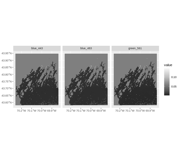
This is neat, but…… it’s dominated by the land. We want to mask the
land. Otherwise, the signal is going to be dominated by land and not
sea. Fortunately, we can use the coastline of the state from the maine
shapefile with mask(). By default, mask keeps what is IN
polygons. So we will need to use the argument
inverse = TRUE. We also need our coastline to have the same
extent as our raster, so, we’ll need to crop it first.
We will also recrop to the AOI again, as our previous crop leaves some cruft around the edges.
R
casco_coastline <- st_crop(maine_borders |> st_make_valid(),
                           aoi_boundary_casco)

# mask and crop
landsat_layers_casco_bay <- mask(landsat_layers_casco,
                                 casco_coastline,
                                 inverse = TRUE) |>
  crop(aoi_boundary_casco)
Did it blend?
R
ggplot() +
  geom_spatraster(data = landsat_layers_casco_bay ) +
  facet_wrap(~lyr) +
  scale_fill_distiller(palette = "Greys", na.value = NA)
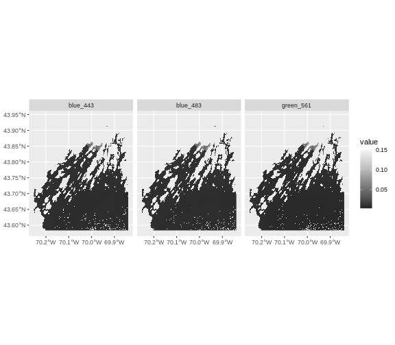
This looks great. There are still some really really high and low
values. We might want to figure out a threshold for clamping. Looking at
the histogram below, something like 0.02 for the upper seems reasonable.
We will use values=FALSE to just remove very high values
and make them NA.
R
# what do things look like?
hist(landsat_layers_casco_bay, breaks = 100, xlim = c(0,0.02))
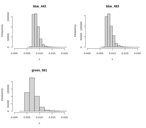
R
#we include lower and upper for good measure
landsat_layers_casco_bay <- clamp(landsat_layers_casco_bay,
                                   lower = 0,
                                   upper = 0.02,
                                   value = FALSE)
Replot it, and, wow, you can really start to see some variability
Two Ways to Perform Raster Calculations
We can calculate with rasters in two different ways:
- by directly using the rasters in R using raster math
or for more efficient processing - particularly if our rasters are large and/or the calculations we are performing are complex:
- using the
lapp()function.
Raster Math & CARI
We can perform raster calculations by subtracting (or adding, multiplying, etc) two rasters. In the geospatial world, we call this “raster math”.
Let’s calculate (green - blue)/(green + blue) to get our CARI score.
After doing this, let’s plot with ggplot.
R
casco_cari <- (landsat_layers_casco_bay$green_561 - landsat_layers_casco_bay$blue_483) /
  (landsat_layers_casco_bay$green_561 + landsat_layers_casco_bay$blue_483)

names(casco_cari) <- "CARI"

ggplot() +
  geom_spatraster(data = casco_cari) +
  scale_fill_viridis_c() +
  labs(fill = "CARI")
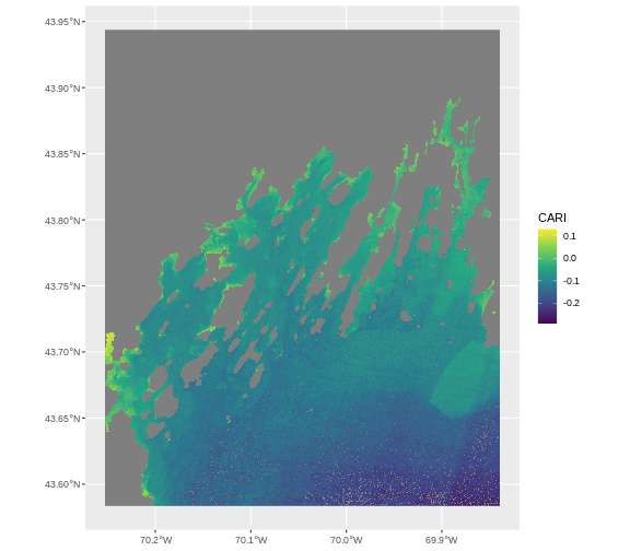
Let’s have a look at the distribution of values in our newly created CARI Model (CHM).
R
hist(casco_cari,
     maxcell = ncell(casco_cari))
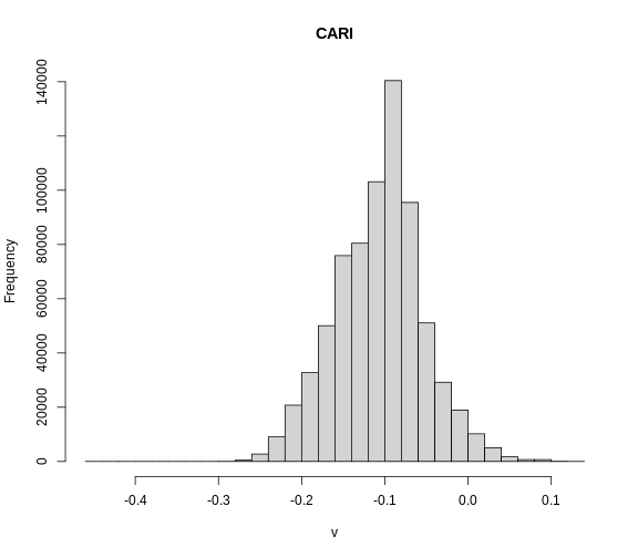
We are definitely starting to see some coastal features here, although whether it is chlorophyll or just coastal runoff is unclear.
Challenge: Explore CHM Raster Values
It’s often a good idea to explore the range of values in a raster dataset just like we might explore a dataset that we collected in the field. Or the spatial distribution to see if it lines up with expectations.
Zoom in on an island (Mackworth if you like). What does the spatial distribution look like? Use
ggplot2orleaflet.Overlay the seagrass bed shapefile. What do you see?
- Zooming in, some of the highest values are close to shorelines.
R
library(leaflet)

leaflet() |>
  addTiles() |>
  addRasterImage(x = casco_cari)
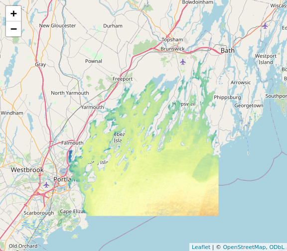
R
library(leaflet)

pal <- colorNumeric("viridis", values(casco_cari), na.color = NA)

leaflet() |>
  addTiles() |>
  addRasterImage(x = casco_cari,
                 colors = pal) |>
  addPolygons(data = seagrass_casco_2022,
               color = "black",
               weight = 1) |>
  addLegend(pal = pal, values = values(casco_cari))
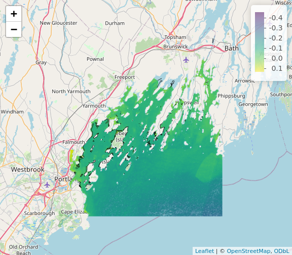
Efficient Raster Calculations
Raster math, like we just did, is an appropriate approach to raster calculations if:
- The rasters we are using are small in size.
- The calculations we are performing are simple.
However, raster math is a less efficient approach as computation becomes more complex or as file sizes become large.
The lapp() function takes two or more rasters and
applies a function to them using efficient processing methods. The
syntax is
outputRaster <- lapp(x, fun=functionName)
In which raster can be either a SpatRaster or a SpatRasterDataset
which is an object that holds rasters. See help(sds).
If you have a raster, stack, you can instead use
app()
outputRaster <- app(x, fun=functionName)
Let’s perform the chla calculation that we calculated above using
raster math, using the app() function.
Data Tip
A custom function consists of a defined set of commands performed on
a input object. Custom functions are particularly useful for tasks that
need to be repeated over and over in the code. A simplified syntax for
writing a custom function in R is:
function_name <- function(variable1, variable2) { WhatYouWantDone, WhatToReturn}
R
get_chl <- function(rast_stack){

  #eqn 3.1
  x <- log10(max(rast_stack[1], rast_stack[2])/rast_stack[3])

  #eqn 3.2
  10^(0.30963 + -2.40052*x + 1.28932*x^2 + 0.52802*x^3 + -1.33825*x^4)
  }

casco_chla <- app(landsat_layers_casco_bay,
                    fun = get_chl)

names(casco_chla) <- "chla"
Now we can plot the CHLa:
R
 ggplot() +
   geom_spatraster(data = casco_chla) +
  scale_fill_viridis_c() +
  labs(fill = "Chl a")
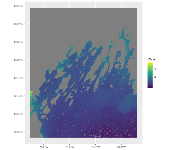
How do the plots of the CHM created with manual raster math and the
lapp() function compare?
Qualitatively, they look about the same!
R
library(leaflet)

pal_chl <- colorNumeric("viridis", values(casco_chla), na.color = NA)

leaflet() |>
  addTiles() |>
  addRasterImage(x = casco_chla,
                 colors = pal_chl) |>
  addPolygons(data = seagrass_casco_2022,
               color = "black",
               weight = 2,
              fill = NA) |>
  addLegend(pal = pal_chl, values = values(casco_chla))
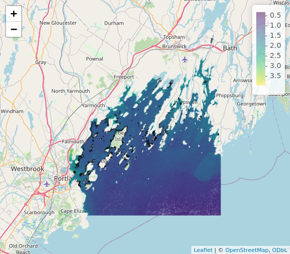
Export a GeoTIFF
Now that we’ve created a new raster, let’s export the data as a
GeoTIFF file using the writeRaster() function.
When we write this raster object to a GeoTIFF file we’ll name it
casco_cari.tif. This name allows us to quickly remember
both what the data contains (CARI data) and for where (Casco bay). The
writeRaster() function by default writes the output file to
your working directory unless you specify a full file path.
We will specify the output format (“GTiff”), the no data value
NAflag = -9999. We will also tell R to overwrite any data
that is already in a file of the same name.
R
writeRaster(casco_cari, "data/casco_cari.tif",
            filetype="GTiff",
            overwrite=TRUE,
            NAflag=-9999)
writeRaster() Options
The function arguments that we used above include:
-
filetype: specify that the format will be
GTiffor GeoTIFF. - overwrite: If TRUE, R will overwrite any existing file with the same name in the specified directory. USE THIS SETTING WITH CAUTION!
-
NAflag: set the GeoTIFF tag for
NoDataValueto -9999, the National Ecological Observatory Network’s (NEON) standardNoDataValue.
