Data frame Manipulation with dplyr
Last updated on 2024-03-12 | Edit this page
Overview
Questions
- How can I manipulate dataframes without repeating myself?
Objectives
- To be able to use the six main dataframe manipulation ‘verbs’ with
pipes in
dplyr. - To understand how
group_by()andsummarize()can be combined to summarize datasets. - Be able to analyze a subset of data using logical filtering.
Let’s begin by loading the Maine DMR kelp-urchin data for the whole coastline.
R
dmr <- read.csv("data/dmr_kelp_urchin.csv")
Manipulation of dataframes means many things to many researchers. We often select certain observations (rows) or variables (columns), we often group the data by a certain variable(s), or we even calculate new variables or summary statistics. We can do these operations using the base R operations we’ve already learned:
R
mean(dmr[dmr$year == 2001, "kelp"])
OUTPUT
[1] 41.36417R
mean(dmr[dmr$year == 2008, "kelp"])
OUTPUT
[1] 55.89091R
mean(dmr[dmr$year == 2014, "kelp"])
OUTPUT
[1] 39.21705But this isn’t very efficient, and can become tedious quickly because there is a fair bit of repetition. Repeating yourself will cost you time, both now and later, and potentially introduce some nasty bugs.
The dplyr package
Luckily, the dplyr package
provides a number of very useful functions for manipulating dataframes
in a way that will reduce the above repetition, reduce the probability
of making errors, and probably even save you some typing. As an added
bonus, you might even find the dplyr grammar easier to
read.
Here we’re going to cover 6 of the most commonly used functions as
well as using pipes (|>) to combine them.
select()filter()group_by()summarize()-
count()andn() mutate()
If you have have not installed this package earlier, please do so:
R
install.packages('dplyr')
Now let’s load the package:
R
library("dplyr")
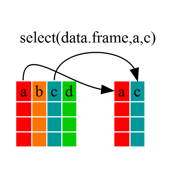
Using select()
If, for example, we wanted to move forward with only a few of the
variables in our dataframe we could use the select()
function. This will keep only the variables you select.
R
dmr_kelp <- select(dmr, year, region, kelp)
If we examine dmr_kelp we’ll see that it only contains
the year, region and kelp columns.
The Pipe
Above we used ‘normal’ grammar, but the strengths of
dplyr lie in combining several functions using pipes. Since
the pipes grammar is unlike anything we’ve seen in R before, let’s
repeat what we’ve done above using pipes.
R
dmr_kelp <- dmr |> select(year, region, kelp)
To help you understand why we wrote that in that way, let’s walk
through it step by step. First we summon the dmr data frame
and pass it on, using the pipe symbol |>, to the next
step, which is the select() function. In this case we don’t
specify which data object we use in the select() function
since in gets that from the previous pipe. Pipes can be used for more
than just dplyr functions. For example, what if we wanted
the unique region names in dmr?
R
dmr$region |> unique()
OUTPUT
[1] "York"          "Casco Bay"     "Midcoast"      "Penobscot Bay"
[5] "MDI"           "Downeast"
We can also chain pipes together. What if we wanted those unique region names sorted?
R
dmr$region |> unique() |> sort()
OUTPUT
[1] "Casco Bay"     "Downeast"      "MDI"           "Midcoast"
[5] "Penobscot Bay" "York"
To make our code more readable when we chain operations together, we often separate each step onto its own line of code.
R
dmr$region |>
  unique() |>
  sort()
This has the secondary benefit that if you’re puzzing through a particularly difficult workflow, you can write it out in comments with one step on each line, and then figure out what functions to use. Like as follows
R
#----
# Step 1: write our what you want to do

# start with regions
  # get the unique values
  # sort them


#----
# Step 2. fill in the first bit

# start with regions
dmr$region
  # get the unique values
  # sort them

#----
# Step 3. fill in the second step after looking up ??unique

# start with regions
dmr$region |>
  # get the unique values
  unique()
  # sort them

#----
# Step 4. Bring it home after googling "how to make alphabetical in R"

# start with regions
dmr$region |>
  # get the unique values
  unique() |>
  # sort them
  sort()
Callout
Fun Fact: You may have encountered pipes before in
other programming contexts. In R, a pipe symbol is |>
while in other contexts it is often | but the concept is
the same!
The |> operator is relatively new in R as part of the
base language. But, the use of pipes has been around for longer.
dplyr and many tidyverse libraries adopted the
pipe from the magrittr
library Danish data scientist Stefan Milton Bache and first released in
2014. You might see %>% in code from experienced R uses
who still use the older style pipe. There are some subtle differences
between the two, but for what we will be doing, |> will
work just fine. Also, Hadley Wickham (the original author of dplyr and
much of the tidyverse who popularized %>%) is pro-base-pipe.
Using filter()
Just as select subsets columns, filter
subsets rows using logical arguments. If we now wanted to move forward
with the above, but only with data from 2011 and kelp data, we can
combine select and filter
R
dmr_2011 <- dmr |>
  filter(year == 2011) |>
  select(year, region, kelp)
R
year_kelp_urchin_dmr <- dmr |>
                           filter(region=="Midcoast") |>
                           select(year,kelp,urchin)

nrow(year_kelp_urchin_dmr)
OUTPUT
[1] 249249 rows, as they are only the Midcoast samples
As with last time, first we pass the dmr dataframe to the
filter() function, then we pass the filtered version of the
dmr data frame to the select() function.
Note: The order of operations is very important in this
case. If we used ‘select’ first, filter would not be able to find the
variable region since we would have removed it in the previous step.
We could now do some specific operations (like calculating summary statistics) on just the Midcoast region.
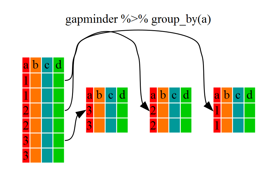
Using group_by() and summarize()
However, we were supposed to be reducing the error prone
repetitiveness of what can be done with base R! If we wanted to do
something for each region, we could take the above approach but we would
have to repeat for each region. Instead of filter(), which
will only pass observations that meet your criteria (in the above:
region==“Midcoast”), we can usegroup_by()`,
which will essentially use every unique criteria that you could have
used in filter.
R
class(dmr)
OUTPUT
[1] "data.frame"R
dmr |> group_by(region) |> class()
OUTPUT
[1] "grouped_df" "tbl_df" "tbl" "data.frame"You will notice that the structure of the dataframe where we used
group_by() (grouped_df) is not the same as the
original dmr (data.frame). A
grouped_df can be thought of as a list where
each item in the listis a data.frame which
contains only the rows that correspond to the a particular value
continent (at least in the example above).
To see this more explicitly, try str() and see the
information about groups at the end.
R
dmr |> group_by(region) |> str()
OUTPUT
gropd_df [1,478 × 15] (S3: grouped_df/tbl_df/tbl/data.frame)
 $ year         : int [1:1478] 2001 2001 2001 2001 2001 2001 2001 2001 2001 2001 ...
 $ region       : chr [1:1478] "York" "York" "York" "York" ...
 $ exposure.code: int [1:1478] 4 4 4 4 4 2 2 3 2 2 ...
 $ coastal.code : int [1:1478] 3 3 3 4 3 2 2 3 2 2 ...
 $ latitude     : num [1:1478] 43.1 43.3 43.4 43.5 43.5 ...
 $ longitude    : num [1:1478] -70.7 -70.6 -70.4 -70.3 -70.3 ...
 $ depth        : int [1:1478] 5 5 5 5 5 5 5 5 5 5 ...
 $ crust        : num [1:1478] 60 75.5 73.5 63.5 72.5 6.1 31.5 31.5 40.5 53 ...
 $ understory   : num [1:1478] 100 100 80 82 69 38.5 74 96.5 60 59.5 ...
 $ kelp         : num [1:1478] 1.9 0 18.5 0.6 63.5 92.5 59 7.7 52.5 29.2 ...
 $ urchin       : num [1:1478] 0 0 0 0 0 0 0 0 0 0 ...
 $ month        : int [1:1478] 6 6 6 6 6 6 6 6 6 6 ...
 $ day          : int [1:1478] 13 13 14 14 14 15 15 15 8 8 ...
 $ survey       : chr [1:1478] "dmr" "dmr" "dmr" "dmr" ...
 $ site         : int [1:1478] 42 47 56 61 62 66 71 70 23 22 ...
 - attr(*, "groups")= tibble [6 × 2] (S3: tbl_df/tbl/data.frame)
  ..$ region: chr [1:6] "Casco Bay" "Downeast" "MDI" "Midcoast" ...
  ..$ .rows : list<int> [1:6]
  .. ..$ : int [1:90] 6 7 8 9 10 11 12 92 93 94 ...
  .. ..$ : int [1:483] 65 66 67 68 69 70 71 72 73 74 ...
  .. ..$ : int [1:342] 44 45 46 47 48 49 50 51 52 53 ...
  .. ..$ : int [1:249] 13 14 15 16 17 18 19 20 21 22 ...
  .. ..$ : int [1:272] 32 33 34 35 36 37 38 39 40 41 ...
  .. ..$ : int [1:42] 1 2 3 4 5 90 91 170 171 172 ...
  .. ..@ ptype: int(0)
  ..- attr(*, ".drop")= logi TRUE
Using summarize()
The above was a bit on the uneventful side but
group_by() is much more exciting in conjunction with
summarize(). This will allow us to create new variable(s)
by using functions that repeat for each of the continent-specific data
frames. That is to say, using the group_by() function, we
split our original dataframe into multiple pieces, then we can run
functions (e.g. mean() or sd()) within
summarize().
R
kelp_by_region <- dmr |>
  group_by(region) |>
  summarize(mean_kelp = mean(kelp))

kelp_by_region
OUTPUT
# A tibble: 6 × 2
  region        mean_kelp
  <chr>             <dbl>
1 Casco Bay          44.1
2 Downeast           67.0
3 MDI                46.9
4 Midcoast           40.5
5 Penobscot Bay      41.1
6 York               19.4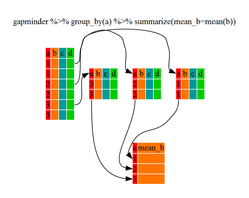
That allowed us to calculate the mean kelp % cover for each region, but it gets even better.
R
urchin_by_region <- dmr |>
   group_by(region) |>
   summarize(mean_urchins = mean(urchin))

urchin_by_region |>
   filter(mean_urchins == min(mean_urchins) | mean_urchins == max(mean_urchins))
OUTPUT
# A tibble: 2 × 2
  region        mean_urchins
  <chr>                <dbl>
1 Casco Bay           0.0767
2 Penobscot Bay       5.30
Another way to do this is to use the dplyr function
arrange(), which arranges the rows in a data frame
according to the order of one or more variables from the data frame. It
has similar syntax to other functions from the dplyr
package. You can use desc() inside arrange()
to sort in descending order.
R
urchin_by_region |>
   arrange(mean_urchins) |>
   head(1)
OUTPUT
# A tibble: 1 × 2
  region    mean_urchins
  <chr>            <dbl>
1 Casco Bay       0.0767
R
urchin_by_region |>
   arrange(desc(mean_urchins)) |>
   head(1)
OUTPUT
# A tibble: 1 × 2
  region        mean_urchins
  <chr>                <dbl>
1 Penobscot Bay         5.30
The function group_by() allows us to group by multiple
variables. Let’s group by year and region.
R
kelp_region_year <- dmr |>
  group_by(region, year) |>
  summarize(mean_kelp = mean(kelp))
OUTPUT
`summarise()` has grouped output by 'region'. You can override using the
`.groups` argument.
That is already quite powerful, but it gets even better! You’re not
limited to defining 1 new variable in summarize().
R
kelp_urchin_region_year <- dmr |>
  group_by(region, year) |>
  summarize(mean_kelp = mean(kelp),
            mean_urchin = mean(urchin),
            sd_kelp = sd(kelp),
            sd_urchin = sd(urchin))
count() and n()
A very common operation is to count the number of observations for
each group. The dplyr package comes with two related
functions that help with this.
For instance, if we wanted to check the number of countries included
in the dataset for the year 2002, we can use the count()
function. It takes the name of one or more columns that contain the
groups we are interested in, and we can optionally sort the results in
descending order by adding sort=TRUE:
R
dmr |>
    filter(year == 2002) |>
    count(region, sort = TRUE)
OUTPUT
         region  n
1      Downeast 25
2           MDI 17
3 Penobscot Bay 15
4      Midcoast 13
5     Casco Bay  8
6          York  2
If we need to use the number of observations in calculations, the
n() function is useful. For instance, if we wanted to get
the standard error of urchins per region:
R
dmr |>
    group_by(region) |>
    summarize(se_urchin = sd(urchin)/sqrt(n()))
OUTPUT
# A tibble: 6 × 2
  region        se_urchin
  <chr>             <dbl>
1 Casco Bay        0.0392
2 Downeast         0.303
3 MDI              0.388
4 Midcoast         0.227
5 Penobscot Bay    0.659
6 York             0.788
Using mutate()
We can also create new variables prior to (or even after) summarizing
information using mutate(). For example, if we wanted to
create a total_fleshy_algae column.
R
dmr |>
  mutate(total_fleshy_algae = kelp + understory)
You can also create a second new column based on the first new column
within the same call of mutate():
R
dmr |>
  mutate(total_fleshy_algae = kelp + understory,
         total_algae = total_fleshy_algae + crust)
Using mutate() and group_by()
together
In some cases, you might want to use mutate() in
conjunction with group_by() to get summarized properties
for groups, but not lose your original data. for example, let’s say we
wanted to calculate how kelp differed from average conditions within a
region each year. This is called an anomaly. In essence we want to get
the average amount of kelp in a region over time, and then calculate a
kelp_anomaly_regional where we subtract the amount of kelp
from the regional average over time. This makes it easier to separate
regional variation from variation over time.
This requires putting mutate() and
group_by() together.
R
dmr |>
  group_by(region) |>
  mutate(mean_kelp_regional = mean(kelp),
         kelp_anomaly_regional = kelp - mean_kelp_regional)
OUTPUT
# A tibble: 1,478 × 17
# Groups:   region [6]
    year region    exposure.code coastal.code latitude longitude depth crust
   <int> <chr>             <int>        <int>    <dbl>     <dbl> <int> <dbl>
 1  2001 York                  4            3     43.1     -70.7     5  60
 2  2001 York                  4            3     43.3     -70.6     5  75.5
 3  2001 York                  4            3     43.4     -70.4     5  73.5
 4  2001 York                  4            4     43.5     -70.3     5  63.5
 5  2001 York                  4            3     43.5     -70.3     5  72.5
 6  2001 Casco Bay             2            2     43.7     -70.1     5   6.1
 7  2001 Casco Bay             2            2     43.8     -70.0     5  31.5
 8  2001 Casco Bay             3            3     43.8     -69.9     5  31.5
 9  2001 Casco Bay             2            2     43.8     -69.9     5  40.5
10  2001 Casco Bay             2            2     43.8     -69.9     5  53
# ℹ 1,468 more rows
# ℹ 9 more variables: understory <dbl>, kelp <dbl>, urchin <dbl>, month <int>,
#   day <int>, survey <chr>, site <int>, mean_kelp_regional <dbl>,
#   kelp_anomaly_regional <dbl>
This worked, but, uh oh. Why is the data frame still grouped? Leaving a data frame grouped will have consequences, as any other mutate will be done by region instead of on the whole data frame. So, for example, if we wanted to then get a global anomaly, i.e., the difference between kelp and the average amount of kelp for the entire data set, we couldn’t just do another set of mutates.
Fortunately, we can resolve this with ungroup(): a
useful verb to insert any time you want to remove all grouping
structure, and are worried dplyr is not doing it for
you.
R
dmr |>
  group_by(region) |>
  mutate(mean_kelp_regional = mean(kelp),
         kelp_anomaly_regional = kelp - mean_kelp_regional) |>
  ungroup() |>
  head()
OUTPUT
# A tibble: 6 × 17
   year region    exposure.code coastal.code latitude longitude depth crust
  <int> <chr>             <int>        <int>    <dbl>     <dbl> <int> <dbl>
1  2001 York                  4            3     43.1     -70.7     5  60
2  2001 York                  4            3     43.3     -70.6     5  75.5
3  2001 York                  4            3     43.4     -70.4     5  73.5
4  2001 York                  4            4     43.5     -70.3     5  63.5
5  2001 York                  4            3     43.5     -70.3     5  72.5
6  2001 Casco Bay             2            2     43.7     -70.1     5   6.1
# ℹ 9 more variables: understory <dbl>, kelp <dbl>, urchin <dbl>, month <int>,
#   day <int>, survey <chr>, site <int>, mean_kelp_regional <dbl>,
#   kelp_anomaly_regional <dbl>
Note, it does convert your data frame into a tibble (a
“tidy” data frame), but if you really want a data frame back, you can
use as.data.frame().
Other great resources
- R for Data Science
- Data Wrangling Cheat sheet
- Introduction to dplyr
- Data wrangling with R and RStudio
Key Points
- Use the
dplyrpackage to manipulate dataframes. - Use
select()to choose variables from a dataframe. - Use
filter()to choose data based on values. - Use
group_by()andsummarize()to work with subsets of data. - Use
count()andn()to obtain the number of observations in columns. - Use
mutate()to create new variables.