Content from Introduction to R and RStudio
Last updated on 2024-03-12 | Edit this page
Overview
Questions
- How to find your way around RStudio?
- How to interact with R?
- How to install packages?
Objectives
- Describe the purpose and use of each pane in the RStudio IDE
- Locate buttons and options in the RStudio IDE
- Define a variable
- Assign data to a variable
- Use mathematical and comparison operators
- Call functions
- Manage packages
Motivation
Science is a multi-step process: once you’ve designed an experiment and collected data, the real fun begins! This lesson will teach you how to start this process using R and RStudio. We will begin with raw data, perform exploratory analyses, and learn how to plot results graphically. This example starts with two datasets on urchins and kelp in Casco Bay and beyond. Can you read the data into R? Can you plot the data or calculate average values for each site? By the end of this set of lessons you will be able to do things like plot the average kelp cover at different areas of Casco Bay in under a minute!
Before Starting The Workshop
Please ensure you have the latest version of R and RStudio installed on your machine. This is important, as some packages used in the workshop may not install correctly (or at all) if R is not up to date.
Introduction to RStudio
Throughout this lesson, we’re going to teach you some of the fundamentals of the R language as well as some best practices for organizing code for scientific projects that will make your life easier.
We’ll be using RStudio: a free, open source R integrated development environment (IDE). It provides a built in editor, works on all platforms (including on servers) and provides many advantages such as integration with version control and project management.
Basic layout
When you first open RStudio, you will be greeted by three panels:
- The interactive R console (entire left)
- Environment/History (tabbed in upper right)
- Files/Plots/Packages/Help/Viewer (tabbed in lower right)
Once you open files, such as R scripts, an editor panel will also open in the top left.
Workflow within RStudio
There are two main ways one can work within RStudio.
- Test and play within the interactive R console then copy code into a .R file to run later.
- This works well when doing small tests and initially starting off.
- It quickly becomes laborious
- Start writing in an .R file and use RStudio’s shortcut keys for the Run command to push the current line, selected lines or modified lines to the interactive R console.
- This is a great way to start; all your code is saved for later
- You will be able to run the file you create from within RStudio or
using R’s
source()function.
Tip: Running segments of your code
RStudio offers you great flexibility in running code from within the editor window. There are buttons, menu choices, and keyboard shortcuts. To run the current line, you can
- click on the
Runbutton above the editor panel, or - select “Run Lines” from the “Code” menu, or
- hit Ctrl+Enter in Windows,
Ctrl+Return in Linux, or
⌘+Return on OS X. (This shortcut can also be seen
by hovering the mouse over the button). To run a block of code, select
it and then
Run. If you have modified a line of code within a block of code you have just run, there is no need to reselect the section andRun, you can use the next button along,Re-run the previous region. This will run the previous code block including the modifications you have made.
Introduction to R
Much of your time in R will be spent in the R interactive console.
This is where you will run all of your code, and can be a useful
environment to try out ideas before adding them to an R script file.
This console in RStudio is the same as the one you would get if you
typed in R in your command-line environment.
The first thing you will see in the R interactive session is a bunch of information, followed by a “>” and a blinking cursor. When you are running a section of your code, this is the location where R will first read your code, attempt to execute them, and then returns a result.
Using R as a calculator
The simplest thing you could do with R is do arithmetic:
R
1 + 100
OUTPUT
[1] 101And R will print out the answer, with a preceding “[1]”.
Don’t worry about this for now, we’ll explain that later. For now think
of it as indicating output.
Like bash, if you type in an incomplete command, R will wait for you to complete it:
OUTPUT
+Any time you hit return and the R session shows a “+”
instead of a “>”, it means it’s waiting for you to
complete the command. If you want to cancel a command you can simply hit
“Esc” and RStudio will give you back the “>”
prompt.
Tip: Cancelling commands
If you’re using R from the command line instead of from within RStudio, you need to use Ctrl+C instead of Esc to cancel the command. This applies to Mac users as well!
Cancelling a command isn’t only useful for killing incomplete commands: you can also use it to tell R to stop running code (for example if it’s taking much longer than you expect), or to get rid of the code you’re currently writing.
When using R as a calculator, the order of operations is the same as you would have learned back in school.
From highest to lowest precedence:
- Parentheses:
(,) - Exponents:
^or** - Divide:
/ - Multiply:
* - Add:
+ - Subtract:
-
R
3 + 5 * 2
OUTPUT
[1] 13Use parentheses to group operations in order to force the order of evaluation if it differs from the default, or to make clear what you intend.
R
(3 + 5) * 2
OUTPUT
[1] 16This can get unwieldy when not needed, but clarifies your intentions. Remember that others may later read your code.
R
(3 + (5 * (2 ^ 2))) # hard to read
3 + 5 * 2 ^ 2       # clear, if you remember the rules
3 + 5 * (2 ^ 2)     # if you forget some rules, this might help
The text after each line of code is called a “comment”. Anything that
follows after the hash (or octothorpe) symbol # is ignored
by R when it executes code.
Really small or large numbers get a scientific notation:
R
2/10000
OUTPUT
[1] 2e-04Which is shorthand for “multiplied by 10^XX”. So
2e-4 is shorthand for 2 * 10^(-4).
You can write numbers in scientific notation too:
R
5e3 # Note the lack of minus here
OUTPUT
[1] 5000Don’t worry about trying to remember every function in R. You can look them up using a search engine, or if you can remember the start of the function’s name, use the tab completion in RStudio.
This is one advantage that RStudio has over R on its own, it has auto-completion abilities that allow you to more easily look up functions, their arguments, and the values that they take.
Typing a ? before the name of a command will open the
help page for that command. As well as providing a detailed description
of the command and how it works, scrolling to the bottom of the help
page will usually show a collection of code examples which illustrate
command usage. We’ll go through an example later.
Comparing things
We can also do comparison in R:
R
1 == 1 # equality (note two equals signs, read as "is equal to")
OUTPUT
[1] TRUER
1 != 2 # inequality (read as "is not equal to")
OUTPUT
[1] TRUER
1 < 2 # less than
OUTPUT
[1] TRUER
1 <= 1 # less than or equal to
OUTPUT
[1] TRUER
1 > 0 # greater than
OUTPUT
[1] TRUER
1 >= -9 # greater than or equal to
OUTPUT
[1] TRUETip: Comparing Numbers
A word of warning about comparing numbers: you should never use
== to compare two numbers unless they are integers (a data
type which can specifically represent only whole numbers).
Computers may only represent decimal numbers with a certain degree of precision, so two numbers which look the same when printed out by R, may actually have different underlying representations and therefore be different by a small margin of error (called Machine numeric tolerance).
Instead you should use the all.equal function.
Further reading: http://floating-point-gui.de/
Variables and assignment
We can store values in variables using the assignment operator
<-, like this:
R
x <- 1/40
Notice that assignment does not print a value. Instead, we stored it
for later in something called a variable.
x now contains the value
0.025:
R
x
OUTPUT
[1] 0.025More precisely, the stored value is a decimal approximation of this fraction called a floating point number.
Look for the Environment tab in one of the panes of
RStudio, and you will see that x and its value have
appeared. Our variable x can be used in place of a number
in any calculation that expects a number:
R
log(x)
OUTPUT
[1] -3.688879Notice also that variables can be reassigned:
R
x <- 100
x used to contain the value 0.025 and and now it has the
value 100.
Assignment values can contain the variable being assigned to:
R
x <- x + 1 #notice how RStudio updates its description of x on the top right tab
y <- x * 2
The right hand side of the assignment can be any valid R expression. The right hand side is fully evaluated before the assignment occurs.
R
mass <- 47.5
This will give a value of 47.5 for the variable mass
R
age <- 122
This will give a value of 122 for the variable age
R
mass <- mass * 2.3
This will multiply the existing value of 47.5 by 2.3 to give a new value of 109.25 to the variable mass.
R
age <- age - 20
This will subtract 20 from the existing value of 122 to give a new value of 102 to the variable age.
One way of answering this question in R is to use the
> to set up the following:
R
mass > age
OUTPUT
[1] TRUEThis should yield a boolean value of TRUE since 109.25 is greater than 102.
Variable names can contain letters, numbers, underscores and periods. They cannot start with a number nor contain spaces at all. Different people use different conventions for long variable names, these include
- periods.between.words
- underscores_between_words
- camelCaseToSeparateWords
What you use is up to you, but be consistent.
It is also possible to use the = operator for
assignment:
R
x = 1/40
But this is much less common among R users. The most important thing
is to be consistent with the operator you use. There
are occasionally places where it is less confusing to use
<- than =, and it is the most common symbol
used in the community. So the recommendation is to use
<-.
The following can be used as R variables:
R
min_height
max.height
MaxLength
celsius2kelvin
The following creates a hidden variable:
R
.mass
We won’t be discussing hidden variables in this lesson. We recommend not using a period at the beginning of variable names unless you intend your variables to be hidden.
The following will not be able to be used to create a variable
Installing Packages
We can use R as a calculator to do mathematical operations (e.g., addition, subtraction, multiplication, division), as we did above. However, we can also use R to carry out more complicated analyses, make visualizations, and much more. In later episodes, we’ll use R to do some data wrangling, plotting, and saving of reformatted data.
R coders around the world have developed collections of R code to accomplish themed tasks (e.g., data wrangling). These collections of R code are known as R packages. It is also important to note that R packages refer to code that is not automatically downloaded when we install R on our computer. Therefore, we’ll have to install each R package that we want to use (more on this below).
We will practice using the dplyr package to wrangle our
datasets in episode 6 and will also practice using the
ggplot2 package to plot our data in episode 7. To give an
example, the dplyr package includes code for a function
called filter(). A function is something that
takes input(s) does some internal operations and produces output(s). For
the filter() function, the inputs are a dataset and a
logical statement (i.e., when data value is greater than or equal to
100) and the output is data within the dataset that has a value greater
than or equal to 100.
There are two main ways to install packages in R:
If you are using RStudio, we can go to
Tools>Install Packages...and then search for the name of the R package we need and clickInstall.We can use the
install.packages( )function. We can do this to install thedplyrR package.
R
install.packages("dplyr")
OUTPUT
The following package(s) will be installed:
- dplyr [1.1.4]
- vctrs [0.6.5]
These packages will be installed into "~/work/r-intro-geospatial/r-intro-geospatial/renv/profiles/lesson-requirements/renv/library/R-4.3/x86_64-pc-linux-gnu".

# Installing packages --------------------------------------------------------
- Installing vctrs ...                          OK [linked from cache]
- Installing dplyr ...                          OK [linked from cache]
Successfully installed 2 packages in 9.1 milliseconds.
It’s important to note that we only need to install the R package on our computer once. Well, if we install a new version of R on the same computer, then we will likely need to also re-install the R packages too.
We would use the following R code to install the ggplot2
package:
R
install.packages("ggplot2")
Now that we’ve installed the R package, we’re ready to use it! To use the R package, we need to “load” it into our R session. We can think of “loading” an R packages as telling R that we’re ready to use the package we just installed. It’s important to note that while we only have to install the package once, we’ll have to load the package each time we open R (or RStudio).
To load an R package, we use the library( ) function. We
can load the dplyr package like this:
R
library(dplyr)
OUTPUT
Attaching package: 'dplyr'OUTPUT
The following objects are masked from 'package:stats':

    filter, lag
OUTPUT
The following objects are masked from 'package:base':

intersect, setdiff, setequal, unionThe correct answers are b and c. Answer a will install, not load, the ggplot2 package. Answer b will correctly load the ggplot2 package. Note there are no quotation marks. Answer c will correctly load the ggplot2 package. Note there are quotation marks. Answer d will produce an error because ggplot2 is misspelled.
Note: It is more common for coders to not use quotation marks when loading an R package (i.e., answer c).
R
library(ggplot2)
Content from Project Management With RStudio
Last updated on 2024-03-12 | Edit this page
Overview
Questions
- How can I manage my projects in R?
Objectives
- Create self-contained projects in RStudio
Introduction
The scientific process is naturally incremental, and many projects start life as random notes, some code, then a manuscript, and eventually everything is a bit mixed together. Organising a project involving spatial data is no different from any other data analysis project, although you may require more disk space than usual.
Managing your projects in a reproducible fashion doesn’t just make your science reproducible, it makes your life easier.
— Vince Buffalo (@vsbuffalo) April 15, 2013
Most people tend to organize their projects like this:
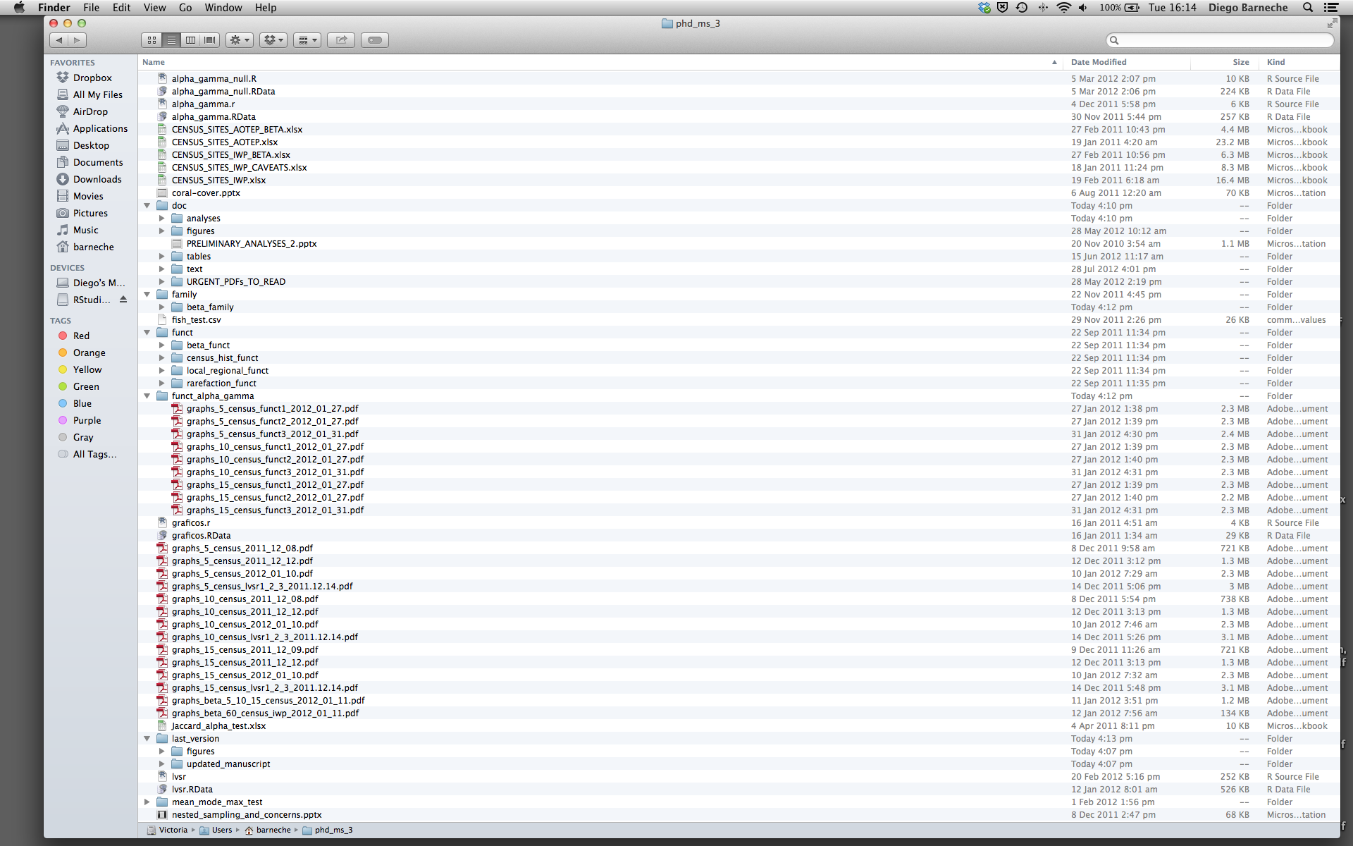
There are many reasons why we should ALWAYS avoid this:
- It is really hard to tell which version of your data is the original and which is the modified;
- It gets really messy because it mixes files with various extensions together;
- It probably takes you a lot of time to actually find things, and relate the correct figures to the exact code that has been used to generate it;
A good project layout will ultimately make your life easier:
- It will help ensure the integrity of your data;
- It makes it simpler to share your code with someone else (a lab-mate, collaborator, or supervisor);
- It allows you to easily upload your code with your manuscript submission;
- It makes it easier to pick the project back up after a break.
A possible solution
Fortunately, there are tools and packages which can help you manage your work effectively.
One of the most powerful and useful aspects of RStudio is its project management functionality. We’ll be using this today to create a self-contained, reproducible project.
A key advantage of an RStudio Project is that whenever we open this
project in subsequent RStudio sessions our working directory will
always be set to the folder r-geospatial. Let’s
check our working directory by entering the following into the R
console:
R
getwd()
R should return your/path/r-geospatial as the working
directory.
Best practices for project organization
Although there is no “best” way to lay out a project, there are some general principles to adhere to that will make project management easier:
Treat data as read only
This is probably the most important goal of setting up a project. Data is typically time consuming and/or expensive to collect. Working with them interactively (e.g., in Excel) where they can be modified means you are never sure of where the data came from, or how it has been modified since collection. It is therefore a good idea to treat your data as “read-only”.
Data Cleaning
In many cases your data will be “dirty”: it will need significant preprocessing to get into a format R (or any other programming language) will find useful. This task is sometimes called “data munging”. I find it useful to store these scripts in a separate folder, and create a second “read-only” data folder to hold the “cleaned” data sets.
Treat generated output as disposable
Anything generated by your scripts should be treated as disposable: it should all be able to be regenerated from your scripts.
There are lots of different ways to manage this output. I find it useful to have an output folder with different sub-directories for each separate analysis. This makes it easier later, as many of my analyses are exploratory and don’t end up being used in the final project, and some of the analyses get shared between projects.
Keep related data together
Some GIS file formats are really 3-6 files that need to be kept together and have the same name, e.g. shapefiles. It may be tempting to store those components separately, but your spatial data will be unusable if you do that.
Keep a consistent naming scheme
It is generally best to avoid renaming downloaded spatial data, so
that a clear connection is maintained with the point of truth. You may
otherwise find yourself wondering whether file_A really is
just a copy of Official_file_on_website or not.
For datasets you generate, it’s worth taking the time to come up with a naming convention that works for your project, and sticking to it. File names don’t have to be long, they just have to be long enough that you can tell what the file is about. Date generated, topic, and whether a product is intermediate or final are good bits of information to keep in a file name. For more tips on naming files, check out the slides from Jenny Bryan’s talk “Naming things” at the 2015 Reproducible Science Workshop.
Tip: Good Enough Practices for Scientific Computing
Good Enough Practices for Scientific Computing gives the following recommendations for project organization:
- Put each project in its own directory, which is named after the project.
- Put text documents associated with the project in the
docdirectory. - Put raw data and metadata in the
datadirectory, and files generated during cleanup and analysis in aresultsdirectory. - Put source for the project’s scripts and programs in the
srcdirectory, and programs brought in from elsewhere or compiled locally in thebindirectory. - Name all files to reflect their content or function.
Save the data in the data directory
Now we have a good directory structure we will now place/save our
data files in the data/ directory.
Challenge 1
1. Download each of the data files listed below (Ctrl+S, right mouse click -> “Save as”, or File -> “Save page as”)
2. Make sure the files have the following names:
dmr_kelp_urchin.csvcasco_kelp_urchin.csvcasco_kelp_urchin_2.csv
3. Save the files in the data/ folder within your
project.
We will load and inspect these data later.
Challenge 2
We also want to move the data that we downloaded from the data
page into a subdirectory inside r-geospatial. If you
haven’t already downloaded the data, you can do so by clicking this download
link.
- Move the downloaded zip file to the
datadirectory. - Once the data have been moved, unzip all files.
Once you have completed moving the data across to the new folder, your data directory should look as follows:
data/
     casco_kelp_urchin.csv
     casco_kelp_urchin_2.csv
     dmr_kelp_urchin.csv
     landsat_casco
     maine_dmr
     maine_gov_maps
     maine_gov_seagrass
modisContent from Data Structures
Last updated on 2024-03-12 | Edit this page
Overview
Questions
- How can I read data in R?
- What are the basic data types in R?
- How do I represent categorical information in R?
Objectives
- To be aware of the different types of data.
- To begin exploring data frames, and understand how they are related to vectors and factors.
- To be able to ask questions from R about the type, class, and structure of an object.
One of R’s most powerful features is its ability to deal with tabular
data, such as you may already have in a spreadsheet or a CSV file. Let’s
start by downloading and reading in a file
casco_kelp_urchin.csv. We will save this data as an object
named casco_dmr:
R
casco_dmr <- read.csv("data/casco_kelp_urchin.csv")
The read.table function is used for reading in tabular
data stored in a text file where the columns of data are separated by
punctuation characters such as tabs (tab-delimited, sometimes with .txt
or .tsv extensions) or commas (comma-delimited values, often with .csv
extensions). For convenience R provides 2 other versions of
read.table. These are: read.csv for files
where the data are separated with commas and read.delim for
files where the data are separated with tabs. Of these three functions
read.csv is the most commonly used. If needed it is
possible to override the default delimiting punctuation marks for both
read.csv and read.delim.
Miscellaneous Tips
- Files can also be downloaded directly from the Internet into a local
folder of your choice onto your computer using the
download.filefunction. Theread.csvfunction can then be executed to read the downloaded file from the download location, for example,
R
download.file("https://cobalt-casco.github.io/r-intro-geospatial/data/casco_kelp_urchin.csv",
              destfile = "data/casco_kelp_urchin.csv")
casco_dmr <- read.csv("data/casco_kelp_urchin.csv")
- Alternatively, you can also read in files directly into R from the
Internet by replacing the file paths with a web address in
read.csv. One should note that in doing this no local copy of the csv file is first saved onto your computer. For example,
R
casco_dmr <- read.csv("https://cobalt-casco.github.io/r-intro-geospatial/data/casco_kelp_urchin.csv")
- You can read directly from excel spreadsheets without converting them to plain text first by using the readxl package.
We can begin exploring our dataset right away, pulling out columns by
specifying them using the $ operator:
R
casco_dmr$year
OUTPUT
 [1] 2001 2001 2001 2001 2001 2001 2001 2002 2002 2002 2002 2002 2002 2002 2002
[16] 2003 2003 2003 2003 2003 2003 2004 2004 2004 2004 2004 2004 2005 2005 2005
[31] 2005 2005 2005 2005 2005 2006 2006 2006 2006 2006 2006 2006 2006 2006 2006
[46] 2007 2007 2007 2007 2007 2007 2007 2008 2008 2008 2008 2008 2008 2009 2009
[61] 2009 2009 2009 2009 2009 2010 2010 2010 2010 2010 2010 2010 2010 2011 2011
[76] 2011 2011 2011 2011 2011 2011 2012 2014 2014 2014 2014 2014 2014 2014 2014
R
casco_dmr$kelp
OUTPUT
 [1]  92.5  59.0   7.7  52.5  29.2 100.0   0.8  87.5  13.0  86.5  96.5  65.0
[13]   5.0   0.0 100.0  64.0  81.0 100.0  56.0  19.5  31.5  55.0  80.5  68.5
[25]  43.0  50.0   9.5  30.0  49.0  79.5  44.5  46.5  24.0  50.5  30.5  42.0
[37]  49.5  51.0  39.0   0.5  71.0  11.0  33.5  75.0  82.5   0.5  35.0   8.5
[49]  55.5  26.0  87.0  32.5   5.0  16.5 100.0  22.0  97.0  39.0   1.5  71.0
[61]  10.5  63.0  73.5  70.5  67.5  17.5   7.5   7.0   0.0  69.5  13.5   2.0
[73]  41.5   7.5  74.5  62.5  76.5  74.5   4.5  71.0   9.5   0.5  46.5  41.5
[85]  55.0  11.0  63.5  14.5  25.5  31.0
We can do other operations on the columns. For example, if we discovered that our data were actually collected two years later:
R
casco_dmr$year + 2
OUTPUT
 [1] 2003 2003 2003 2003 2003 2003 2003 2004 2004 2004 2004 2004 2004 2004 2004
[16] 2005 2005 2005 2005 2005 2005 2006 2006 2006 2006 2006 2006 2007 2007 2007
[31] 2007 2007 2007 2007 2007 2008 2008 2008 2008 2008 2008 2008 2008 2008 2008
[46] 2009 2009 2009 2009 2009 2009 2009 2010 2010 2010 2010 2010 2010 2011 2011
[61] 2011 2011 2011 2011 2011 2012 2012 2012 2012 2012 2012 2012 2012 2013 2013
[76] 2013 2013 2013 2013 2013 2013 2014 2016 2016 2016 2016 2016 2016 2016 2016
As an aside, did this change the original year data? How would you check?
But what about:
R
casco_dmr$year + casco_dmr$region
ERROR
Error in casco_dmr$year + casco_dmr$region: non-numeric argument to binary operatorUnderstanding what happened here is key to successfully analyzing data in R.
Data Types
If you guessed that the last command will return an error because
2008 plus "Casco Bay" is nonsense, you’re
right - and you already have some intuition for an important concept in
programming called data classes. We can ask what class of data
something is:
R
class(casco_dmr$year)
OUTPUT
[1] "integer"There are 6 main types: numeric, integer,
complex, logical, character, and
factor.
R
class(3.14)
OUTPUT
[1] "numeric"R
class(1L) # The L suffix forces the number to be an integer, since by default R uses float numbers
OUTPUT
[1] "integer"R
class(1+1i)
OUTPUT
[1] "complex"R
class(TRUE)
OUTPUT
[1] "logical"R
class('banana')
OUTPUT
[1] "character"R
class(factor('banana'))
OUTPUT
[1] "factor"The types numeric, integer, and
complex are all numbers, although they are stored
differently and have different mathematical properties.
logical type data include only TRUE and
FALSE values, while character type data can
contain any kind of characters. Finally, factor is a
special type that was built to help us store categorical variables,
variables that have a fixed and known set of possible values. We’ll talk
more about them in a little bit.
No matter how complicated our analyses become, all data in R is interpreted a specific data class. This strictness has some really important consequences.
Let’s say that a collaborator sends you an updated data file named
data/casco_kelp_urchin_2.csv.
Load the new data file as casco_dmr_2, and check what
class of data we find in the year column:
R
casco_dmr_2 <- read.csv("data/casco_kelp_urchin_2.csv")
class(casco_dmr_2$year)
OUTPUT
[1] "character"Oh no, our year data aren’t the numeric type anymore! If we try to do the same math we did on them before, we run into trouble:
R
casco_dmr_2$year + 2
ERROR
Error in casco_dmr_2$year + 2: non-numeric argument to binary operatorWhat happened? When R reads a csv file into one of these tables, it insists that everything in a column be the same class; if it can’t understand everything in the column as numeric, then nothing in the column gets to be numeric. The table that R loaded our data into is something called a dataframe, and it is our first example of something called a data structure, that is, a structure which R knows how to build out of the basic data types.
We can see that it is a dataframe by calling the class()
function on it:
R
class(casco_dmr)
OUTPUT
[1] "data.frame"In order to successfully use our data in R, we need to understand what the basic data structures are, and how they behave. Note: in this lesson we will not cover lists, which are a basic data structure in R. You can learn more about them here.
Vectors and Type Coercion
To better understand this behavior, let’s meet another of the data structures: the vector.
R
my_vector <- vector(length = 3)
my_vector
OUTPUT
[1] FALSE FALSE FALSEA vector in R is essentially an ordered list of things, with the
special condition that everything in the vector must be the same basic
data type. If you don’t choose the data type, it’ll default to
logical; or, you can declare an empty vector of whatever
type you like.
R
another_vector <- vector(mode = 'character', length = 3)
another_vector
OUTPUT
[1] "" "" ""You can check if something is a vector:
R
str(another_vector)
OUTPUT
chr [1:3] "" "" ""The somewhat cryptic output from this command indicates the basic
data type found in this vector (in this case chr or
character), an indication of the number of things in the vector (the
indexes of the vector, in this case: [1:3]), and a few
examples of what’s actually in the vector (in this case empty character
strings). If we similarly do:
R
str(casco_dmr$year)
OUTPUT
int [1:90] 2001 2001 2001 2001 2001 2001 2001 2002 2002 2002 ...we see that casco_dmr$year is a vector, too! The columns
of data we load into R data frames are all vectors, and that’s the root
of why R forces everything in a column to be the same basic data
type.
Discussion 1
Why is R so opinionated about what we put in our columns of data? How does this help us?
By keeping everything in a column the same, we allow ourselves to make simple assumptions about our data; if you can interpret one entry in the column as a number, then you can interpret all of them as numbers, so we don’t have to check every time. This consistency is what people mean when they talk about clean data; in the long run, strict consistency goes a long way to making our lives easier in R.
You can also make vectors with explicit contents with the combine function:
R
combine_vector <- c(2, 6, 3)
combine_vector
OUTPUT
[1] 2 6 3We can see what is at a certain index of a vector using the
[] notation. For example, what is the second element of
combine_vector?
R
combine_vector[2]
OUTPUT
[1] 6Type Coercion
Given what we’ve learned so far, what do you think the following will produce?
R
quiz_vector <- c(2, 6, '3')
This is something called type coercion, and it is the source of many surprises and the reason why we need to be aware of the basic data types and how R will interpret them. When R encounters a mix of types (here numeric and character) to be combined into a single vector, it will force them all to be the same type. Consider:
R
coercion_vector <- c('a', TRUE)
coercion_vector
OUTPUT
[1] "a" "TRUE"R
another_coercion_vector <- c(0, TRUE)
another_coercion_vector
OUTPUT
[1] 0 1The coercion rules go: logical ->
integer -> numeric ->
complex -> character, where -> can be
read as are transformed into. You can try to force coercion
against this flow using the as. functions:
R
character_vector_example <- c('0', '2', '4')
character_vector_example
OUTPUT
[1] "0" "2" "4"R
character_coerced_to_numeric <- as.numeric(character_vector_example)
character_coerced_to_numeric
OUTPUT
[1] 0 2 4R
numeric_coerced_to_logical <- as.logical(character_coerced_to_numeric)
numeric_coerced_to_logical
OUTPUT
[1] FALSE TRUE TRUEAs you can see, some surprising things can happen when R forces one basic data type into another! Nitty-gritty of type coercion aside, the point is: if your data doesn’t look like what you thought it was going to look like, type coercion may well be to blame; make sure everything is the same type in your vectors and your columns of data frames, or you will get nasty surprises!
R
str(casco_dmr$year)
OUTPUT
int [1:90] 2001 2001 2001 2001 2001 2001 2001 2002 2002 2002 ...R
str(casco_dmr_2$year)
OUTPUT
chr [1:90] "year 2001" "2001" "2001" "2001" "2001" "2001" "2001" "2002" ...The data in casco_dmr_2$year is stored as a character
vector, rather than as a numeric vector. This is because of the “year”
character string in the first data point.
The combine function, c(), will also append things to an
existing vector:
R
ab_vector <- c('a', 'b')
ab_vector
OUTPUT
[1] "a" "b"R
combine_example <- c(ab_vector, 'DC')
combine_example
OUTPUT
[1] "a" "b" "DC"You can also make series of numbers:
R
my_series <- 1:10
my_series
OUTPUT
[1] 1 2 3 4 5 6 7 8 9 10R
seq(10)
OUTPUT
[1] 1 2 3 4 5 6 7 8 9 10R
seq(1,10, by = 0.1)
OUTPUT
 [1]  1.0  1.1  1.2  1.3  1.4  1.5  1.6  1.7  1.8  1.9  2.0  2.1  2.2  2.3  2.4
[16]  2.5  2.6  2.7  2.8  2.9  3.0  3.1  3.2  3.3  3.4  3.5  3.6  3.7  3.8  3.9
[31]  4.0  4.1  4.2  4.3  4.4  4.5  4.6  4.7  4.8  4.9  5.0  5.1  5.2  5.3  5.4
[46]  5.5  5.6  5.7  5.8  5.9  6.0  6.1  6.2  6.3  6.4  6.5  6.6  6.7  6.8  6.9
[61]  7.0  7.1  7.2  7.3  7.4  7.5  7.6  7.7  7.8  7.9  8.0  8.1  8.2  8.3  8.4
[76]  8.5  8.6  8.7  8.8  8.9  9.0  9.1  9.2  9.3  9.4  9.5  9.6  9.7  9.8  9.9
[91] 10.0
We can ask a few questions about vectors:
R
sequence_example <- seq(10)
head(sequence_example,n = 2)
OUTPUT
[1] 1 2R
tail(sequence_example, n = 4)
OUTPUT
[1] 7 8 9 10R
length(sequence_example)
OUTPUT
[1] 10R
class(sequence_example)
OUTPUT
[1] "integer"Finally, you can give names to elements in your vector:
R
my_example <- 5:8
names(my_example) <- c("a", "b", "c", "d")
my_example
OUTPUT
a b c d
5 6 7 8
R
names(my_example)
OUTPUT
[1] "a" "b" "c" "d"R
x <- 1:26
x <- x * 2
names(x) <- LETTERS
Factors
We said that columns in data frames were vectors:
R
str(casco_dmr$year)
OUTPUT
int [1:90] 2001 2001 2001 2001 2001 2001 2001 2002 2002 2002 ...R
str(casco_dmr$kelp)
OUTPUT
num [1:90] 92.5 59 7.7 52.5 29.2 100 0.8 87.5 13 86.5 ...R
str(casco_dmr$region)
OUTPUT
chr [1:90] "Casco Bay" "Casco Bay" "Casco Bay" "Casco Bay" "Casco Bay" ...One final important data structure in R is called a “factor” (that special data type we mentioned above). Factors look like character data, but are used to represent data where each element of the vector must be one of a limited number of “levels”. To phrase that another way, factors are an “enumerated” type where there are a finite number of pre-defined values that your vector can have.
For example, let’s make a character vector with all the sampling regions in the DMR kelp data:
R
maine_regions <- c("York", "Casco Bay", "Midcoast", "Penobscot Bay", "MDI", "Downeast")
maine_regions
OUTPUT
[1] "York"          "Casco Bay"     "Midcoast"      "Penobscot Bay"
[5] "MDI"           "Downeast"
R
class(maine_regions)
OUTPUT
[1] "character"R
str(maine_regions)
OUTPUT
chr [1:6] "York" "Casco Bay" "Midcoast" "Penobscot Bay" "MDI" "Downeast"We can turn a vector into a factor like so:
R
me_region_factor <- factor(maine_regions)
class(me_region_factor)
OUTPUT
[1] "factor"R
str(me_region_factor)
OUTPUT
Factor w/ 6 levels "Casco Bay","Downeast",..: 6 1 4 5 3 2Now R has noticed that there are 6 possible categories in our data, but it also did something surprising. Instead of printing out the strings we gave it, we got a bunch of numbers instead. R has replaced our human-readable categories with numbered indices under the hood! This is necessary as many statistical calculations utilize such numerical representations for categorical data.
Challenge 3
Convert the region column of our casco_dmr
data frame to a factor. Then try converting it back to a character
vector.
Now try converting year in our casco_dmr
data frame to a factor, then back to a numeric vector. What happens if
you use as.numeric()?
Remember that you can always reload the casco_dmr data
frame using read.csv("data/casco_kelp_urchin.csv") if you
accidentally mess up your data!
Converting character vectors to factors can be done using the
factor() function:
R
casco_dmr$region <- factor(casco_dmr$region)
casco_dmr$region
OUTPUT
 [1] Casco Bay Casco Bay Casco Bay Casco Bay Casco Bay Casco Bay Casco Bay
 [8] Casco Bay Casco Bay Casco Bay Casco Bay Casco Bay Casco Bay Casco Bay
[15] Casco Bay Casco Bay Casco Bay Casco Bay Casco Bay Casco Bay Casco Bay
[22] Casco Bay Casco Bay Casco Bay Casco Bay Casco Bay Casco Bay Casco Bay
[29] Casco Bay Casco Bay Casco Bay Casco Bay Casco Bay Casco Bay Casco Bay
[36] Casco Bay Casco Bay Casco Bay Casco Bay Casco Bay Casco Bay Casco Bay
[43] Casco Bay Casco Bay Casco Bay Casco Bay Casco Bay Casco Bay Casco Bay
[50] Casco Bay Casco Bay Casco Bay Casco Bay Casco Bay Casco Bay Casco Bay
[57] Casco Bay Casco Bay Casco Bay Casco Bay Casco Bay Casco Bay Casco Bay
[64] Casco Bay Casco Bay Casco Bay Casco Bay Casco Bay Casco Bay Casco Bay
[71] Casco Bay Casco Bay Casco Bay Casco Bay Casco Bay Casco Bay Casco Bay
[78] Casco Bay Casco Bay Casco Bay Casco Bay Casco Bay Casco Bay Casco Bay
[85] Casco Bay Casco Bay Casco Bay Casco Bay Casco Bay Casco Bay
Levels: Casco Bay
You can convert these back to character vectors using
as.character():
R
casco_dmr$region <- as.character(casco_dmr$region)
casco_dmr$region
OUTPUT
 [1] "Casco Bay" "Casco Bay" "Casco Bay" "Casco Bay" "Casco Bay" "Casco Bay"
 [7] "Casco Bay" "Casco Bay" "Casco Bay" "Casco Bay" "Casco Bay" "Casco Bay"
[13] "Casco Bay" "Casco Bay" "Casco Bay" "Casco Bay" "Casco Bay" "Casco Bay"
[19] "Casco Bay" "Casco Bay" "Casco Bay" "Casco Bay" "Casco Bay" "Casco Bay"
[25] "Casco Bay" "Casco Bay" "Casco Bay" "Casco Bay" "Casco Bay" "Casco Bay"
[31] "Casco Bay" "Casco Bay" "Casco Bay" "Casco Bay" "Casco Bay" "Casco Bay"
[37] "Casco Bay" "Casco Bay" "Casco Bay" "Casco Bay" "Casco Bay" "Casco Bay"
[43] "Casco Bay" "Casco Bay" "Casco Bay" "Casco Bay" "Casco Bay" "Casco Bay"
[49] "Casco Bay" "Casco Bay" "Casco Bay" "Casco Bay" "Casco Bay" "Casco Bay"
[55] "Casco Bay" "Casco Bay" "Casco Bay" "Casco Bay" "Casco Bay" "Casco Bay"
[61] "Casco Bay" "Casco Bay" "Casco Bay" "Casco Bay" "Casco Bay" "Casco Bay"
[67] "Casco Bay" "Casco Bay" "Casco Bay" "Casco Bay" "Casco Bay" "Casco Bay"
[73] "Casco Bay" "Casco Bay" "Casco Bay" "Casco Bay" "Casco Bay" "Casco Bay"
[79] "Casco Bay" "Casco Bay" "Casco Bay" "Casco Bay" "Casco Bay" "Casco Bay"
[85] "Casco Bay" "Casco Bay" "Casco Bay" "Casco Bay" "Casco Bay" "Casco Bay"
You can convert numeric vectors to factors in the exact same way:
R
casco_dmr$year <- factor(casco_dmr$year)
casco_dmr$year
OUTPUT
 [1] 2001 2001 2001 2001 2001 2001 2001 2002 2002 2002 2002 2002 2002 2002 2002
[16] 2003 2003 2003 2003 2003 2003 2004 2004 2004 2004 2004 2004 2005 2005 2005
[31] 2005 2005 2005 2005 2005 2006 2006 2006 2006 2006 2006 2006 2006 2006 2006
[46] 2007 2007 2007 2007 2007 2007 2007 2008 2008 2008 2008 2008 2008 2009 2009
[61] 2009 2009 2009 2009 2009 2010 2010 2010 2010 2010 2010 2010 2010 2011 2011
[76] 2011 2011 2011 2011 2011 2011 2012 2014 2014 2014 2014 2014 2014 2014 2014
Levels: 2001 2002 2003 2004 2005 2006 2007 2008 2009 2010 2011 2012 2014
But be careful – you can’t use as.numeric() to convert
factors to numerics!
R
as.numeric(casco_dmr$year)
OUTPUT
 [1]  1  1  1  1  1  1  1  2  2  2  2  2  2  2  2  3  3  3  3  3  3  4  4  4  4
[26]  4  4  5  5  5  5  5  5  5  5  6  6  6  6  6  6  6  6  6  6  7  7  7  7  7
[51]  7  7  8  8  8  8  8  8  9  9  9  9  9  9  9 10 10 10 10 10 10 10 10 11 11
[76] 11 11 11 11 11 11 12 13 13 13 13 13 13 13 13
Instead, as.numeric() converts factors to those “numbers
under the hood” we talked about. To go from a factor to a number, you
need to first turn the factor into a character vector, and then
turn that into a numeric vector:
R
casco_dmr$year <- as.character(casco_dmr$year)
casco_dmr$year <- as.numeric(casco_dmr$year)
casco_dmr$year
OUTPUT
 [1] 2001 2001 2001 2001 2001 2001 2001 2002 2002 2002 2002 2002 2002 2002 2002
[16] 2003 2003 2003 2003 2003 2003 2004 2004 2004 2004 2004 2004 2005 2005 2005
[31] 2005 2005 2005 2005 2005 2006 2006 2006 2006 2006 2006 2006 2006 2006 2006
[46] 2007 2007 2007 2007 2007 2007 2007 2008 2008 2008 2008 2008 2008 2009 2009
[61] 2009 2009 2009 2009 2009 2010 2010 2010 2010 2010 2010 2010 2010 2011 2011
[76] 2011 2011 2011 2011 2011 2011 2012 2014 2014 2014 2014 2014 2014 2014 2014
Note: new students find the help files difficult to understand; make sure to let them know that this is typical, and encourage them to take their best guess based on semantic meaning, even if they aren’t sure.
When doing statistical modelling, it’s important to know what the baseline levels are. This is assumed to be the first factor, but by default factors are labeled in alphabetical order. You can change this by specifying the levels:
R
treatment <- c("case", "control", "control", "case")
factor_ordering_example <- factor(treatment, levels = c("control", "case"))
str(factor_ordering_example)
OUTPUT
Factor w/ 2 levels "control","case": 2 1 1 2In this case, we’ve explicitly told R that “control” should represented by 1, and “case” by 2. This designation can be very important for interpreting the results of statistical models!
To know what the levels map to, we can use levels() for
factors. To do the same for characters, we can use
unique().
R
levels(factor_ordering_example)
OUTPUT
[1] "control" "case" R
unique(maine_regions)
OUTPUT
[1] "York"          "Casco Bay"     "Midcoast"      "Penobscot Bay"
[5] "MDI"           "Downeast"
Note that the order is different! For unique(), it’s
based on the order of observation in the vector. For levels, it’s been
set. If we want to sort from unique(), which can be very
useful, we can try:
R
non_alpha_vector <- c("b", "a", "c")

unique(non_alpha_vector)
OUTPUT
[1] "b" "a" "c"R
sort(unique(non_alpha_vector) )
OUTPUT
[1] "a" "b" "c"Content from Subsetting Data
Last updated on 2024-03-12 | Edit this page
Overview
Questions
- How can I work with subsets of data in R?
Objectives
- To be able to subset vectors and data frames
- To be able to extract individual and multiple elements: by index, by name, using comparison operations
- To be able to skip and remove elements from various data structures.
R has many powerful subset operators. Mastering them will allow you to easily perform complex operations on any kind of dataset.
There are six different ways we can subset any kind of object, and three different subsetting operators for the different data structures. Why so many? Well, this gives us a lot of flexibility that can come in useful. At first, though, it may seem overwhelming. Don’t worry!
Let’s start with the workhorse of R: a simple numeric vector.
R
x <- c(5.4, 6.2, 7.1, 4.8, 7.5)
names(x) <- c('a', 'b', 'c', 'd', 'e')
x
OUTPUT
  a   b   c   d   e
5.4 6.2 7.1 4.8 7.5 So now that we’ve created a dummy vector to play with, how do we get at its contents?
Accessing elements using their indices
To extract elements of a vector we can give their corresponding index, or their numbered place in the vector starting from one:
R
x[1]
OUTPUT
  a
5.4
R
x[4]
OUTPUT
  d
4.8
It may look different, but the square brackets operator is a function. For vectors (and matrices), it means “get me the nth element”.
We can ask for multiple elements at once:
R
x[c(1, 3)]
OUTPUT
  a   c
5.4 7.1
Or slices of the vector:
R
x[1:4]
OUTPUT
  a   b   c   d
5.4 6.2 7.1 4.8
the : operator creates a sequence of numbers from the
left element to the right.
R
1:4
OUTPUT
[1] 1 2 3 4R
c(1, 2, 3, 4)
OUTPUT
[1] 1 2 3 4We can ask for the same element multiple times:
R
x[c(1, 1, 3)]
OUTPUT
  a   a   c
5.4 5.4 7.1
If we ask for an index beyond the length of the vector, R will return a missing value:
R
x[6]
OUTPUT
<NA>
  NA
This is a vector of length one containing an NA, whose
name is also NA. Here NA stands for “Not
Available”, and is a common way to represent a missing value.
If we ask for the 0th element, we get an empty vector:
R
x[0]
OUTPUT
named numeric(0)Skipping and removing elements
If we use a negative number as the index of a vector, R will return every element except for the one specified:
R
x[-2]
OUTPUT
  a   c   d   e
5.4 7.1 4.8 7.5
We can skip multiple elements:
R
x[c(-1, -5)] # or x[-c(1,5)]
OUTPUT
  b   c   d
6.2 7.1 4.8
Tip: Order of operations
A common trip up for novices occurs when trying to skip slices of a vector. It’s natural to to try to negate a sequence like so:
R
x[-1:3]
This gives a somewhat cryptic error:
ERROR
Error in x[-1:3]: only 0's may be mixed with negative subscriptsBut remember the order of operations. : is really a
function. It takes its first argument as -1, and its second as 3, so
generates the sequence of numbers: c(-1, 0, 1, 2, 3).
The correct solution is to wrap that function call in brackets, so
that the - operator applies to the result:
R
x[-(1:3)]
OUTPUT
  d   e
4.8 7.5
To remove elements from a vector, we need to assign the result back into the variable:
R
x <- x[-4]
x
OUTPUT
  a   b   c   e
5.4 6.2 7.1 7.5
Challenge 1
Given the following code:
R
x <- c(5.4, 6.2, 7.1, 4.8, 7.5)
names(x) <- c('a', 'b', 'c', 'd', 'e')
print(x)
OUTPUT
  a   b   c   d   e
5.4 6.2 7.1 4.8 7.5
Come up with at least 3 different commands that will produce the following output:
OUTPUT
  b   c   d
6.2 7.1 4.8
After you find 3 different commands, compare notes with your neighbour. Did you have different strategies?
R
x[2:4]
OUTPUT
  b   c   d
6.2 7.1 4.8
R
x[-c(1,5)]
OUTPUT
  b   c   d
6.2 7.1 4.8
R
x[c("b", "c", "d")]
OUTPUT
  b   c   d
6.2 7.1 4.8
R
x[c(2,3,4)]
OUTPUT
  b   c   d
6.2 7.1 4.8
Subsetting by name
We can extract elements by using their name, instead of extracting by index:
R
x <- c(a = 5.4, b = 6.2, c = 7.1, d = 4.8, e = 7.5) # we can name a vector 'on the fly'
x[c("a", "c")]
OUTPUT
  a   c
5.4 7.1
This is usually a much more reliable way to subset objects: the position of various elements can often change when chaining together subsetting operations, but the names will always remain the same!
Subsetting through other logical operations
We can also use any logical vector to subset:
R
x[c(FALSE, FALSE, TRUE, FALSE, TRUE)]
OUTPUT
  c   e
7.1 7.5
Since comparison operators (e.g. >,
<, ==) evaluate to logical vectors, we can
also use them to succinctly subset vectors: the following statement
gives the same result as the previous one.
R
x[x > 7]
OUTPUT
  c   e
7.1 7.5
Breaking it down, this statement first evaluates
x > 7, generating a logical vector
c(FALSE, FALSE, TRUE, FALSE, TRUE), and then selects the
elements of x corresponding to the TRUE
values.
We can use == to mimic the previous method of indexing
by name (you have to use == rather than = for
comparisons, as R has another use for =):
R
x[names(x) == "a"]
OUTPUT
  a
5.4
Tip: Combining logical conditions
We often want to combine multiple logical criteria. For example, we might want to find all the plots that are located in Casco Bay or Penobscot Bay and have urchin densities within a certain range. Several operations for combining logical vectors exist in R:
-
&, the “logical AND” operator: returnsTRUEif both the left and right areTRUE. -
|, the “logical OR” operator: returnsTRUE, if either the left or right (or both) areTRUE.
You may sometimes see && and ||
instead of & and |. These two-character
operators only look at the first element of each vector and ignore the
remaining elements. In general you should not use the two-character
operators in data analysis; save them for programming, i.e. deciding
whether to execute a statement.
-
!, the “logical NOT” operator: convertsTRUEtoFALSEandFALSEtoTRUE. It can negate a single logical condition (eg!TRUEbecomesFALSE), or a whole vector of conditions(eg!c(TRUE, FALSE)becomesc(FALSE, TRUE)).
Additionally, you can compare the elements within a single vector
using the all function (which returns TRUE if
every element of the vector is TRUE) and the
any function (which returns TRUE if one or
more elements of the vector are TRUE).
R
x_subset <- x[x<7 & x>4]
print(x_subset)
OUTPUT
  a   b   d
5.4 6.2 4.8
Skipping named elements
Skipping or removing named elements is a little harder. If we try to skip one named element by negating the string, R complains (slightly obscurely) that it doesn’t know how to take the negative of a string:
R
x <- c(a=5.4, b=6.2, c=7.1, d=4.8, e=7.5) # we start again by naming a vector 'on the fly'
x[-"a"]
ERROR
Error in -"a": invalid argument to unary operatorHowever, we can use the != (not-equals) operator to
construct a logical vector that will do what we want:
R
x[names(x) != "a"]
OUTPUT
  b   c   d   e
6.2 7.1 4.8 7.5
Skipping multiple named indices is a little bit harder still. Suppose
we want to drop the "a" and "c" elements, so
we try this:
R
x[names(x)!=c("a","c")]
WARNING
Warning in names(x) != c("a", "c"): longer object length is not a multiple of
shorter object length
OUTPUT
  b   c   d   e
6.2 7.1 4.8 7.5
R did something, but it gave us a warning that we ought to
pay attention to, and it apparently gave us the wrong answer
(the "c" element is still included in the vector)!
So what does != actually do in this case? That’s an
excellent question.
Recycling
Let’s take a look at the comparison component of this code:
R
names(x) != c("a", "c")
WARNING
Warning in names(x) != c("a", "c"): longer object length is not a multiple of
shorter object length
OUTPUT
[1] FALSE TRUE TRUE TRUE TRUEWhy does R give TRUE as the third element of this
vector, when names(x)[3] != "c" is obviously false? When
you use !=, R tries to compare each element of the left
argument with the corresponding element of its right argument. What
happens when you compare vectors of different lengths?
When one vector is shorter than the other, it gets recycled.
In this case R repeats c("a", "c") as many
times as necessary to match names(x), i.e. we get
c("a","c","a","c","a"). Since the recycled "a"
doesn’t match the third element of names(x), the value of
!= is TRUE. Because in this case the longer
vector length (5) isn’t a multiple of the shorter vector length (2), R
printed a warning message. If we had been unlucky and
names(x) had contained six elements, R would
silently have done the wrong thing (i.e., not what we intended
it to do). This recycling rule can can introduce hard-to-find and subtle
bugs!
The way to get R to do what we really want (match each
element of the left argument with all of the elements of the
right argument) it to use the %in% operator. The
%in% operator goes through each element of its left
argument, in this case the names of x, and asks, “Does this
element occur in the second argument?”. Here, since we want to
exclude values, we also need a ! operator to
change “in” to “not in”:
R
x[! names(x) %in% c("a","c") ]
OUTPUT
  b   d   e
6.2 4.8 7.5 Handling special values
At some point you will encounter functions in R that cannot handle missing, infinite, or undefined data.
There are a number of special functions you can use to filter out this data:
-
is.nawill return all positions in a vector, matrix, or data frame containingNA(orNaN) - likewise,
is.nan, andis.infinitewill do the same forNaNandInf. -
is.finitewill return all positions in a vector, matrix, or data.frame that do not containNA,NaNorInf. -
na.omitwill filter out all missing values from a vector
Data frames
Data frames are two dimensional objects (under the hood they are structured as lists in R, but we aren’t going to go into detail on that). Data frames have some useful subsetting operators.
Let’s look at the Casco Bay DMR kelp-urchin data again.
R
casco_dmr <- read.csv("data/casco_kelp_urchin.csv") # if you don't already have the data loaded
[ with one argument will extract a column - each element
of the data frame corresponds to a column. The resulting object will be
a data frame:
R
head(casco_dmr[3])
OUTPUT
  exposure.code
1             2
2             2
3             3
4             2
5             2
6             1
R
class(casco_dmr[3])
OUTPUT
[1] "data.frame"Similarly, [[ will act to extract a single
column:
R
head(casco_dmr[["exposure.code"]])
OUTPUT
[1] 2 2 3 2 2 1And $ provides a convenient shorthand to extract columns
by name:
R
head(casco_dmr$exposure.code)
OUTPUT
[1] 2 2 3 2 2 1To select specific rows and/or columns, you can provide two arguments
to [. The first identifies the rows to subset, and the
second the columns.
R
casco_dmr[1:3, ]
OUTPUT
  year    region exposure.code coastal.code latitude longitude depth crust
1 2001 Casco Bay             2            2 43.72766 -70.10721     5   6.1
2 2001 Casco Bay             2            2 43.76509 -69.96087     5  31.5
3 2001 Casco Bay             3            3 43.75199 -69.93420     5  31.5
  understory kelp urchin month day survey site
1       38.5 92.5      0     6  15    dmr   66
2       74.0 59.0      0     6  15    dmr   71
3       96.5  7.7      0     6  15    dmr   70
If we subset a single row, the result will be a data frame (because the elements are mixed types):
R
casco_dmr[3, ]
OUTPUT
  year    region exposure.code coastal.code latitude longitude depth crust
3 2001 Casco Bay             3            3 43.75199  -69.9342     5  31.5
  understory kelp urchin month day survey site
3       96.5  7.7      0     6  15    dmr   70
But for a single column the result will be a vector (this can be
changed with the argument, drop = FALSE).
R
str(casco_dmr[, 3])
OUTPUT
int [1:90] 2 2 3 2 2 1 2 3 3 5 ...R
str(casco_dmr[, 3, drop = FALSE])
OUTPUT
'data.frame':	90 obs. of  1 variable:
 $ exposure.code: int  2 2 3 2 2 1 2 3 3 5 ...
Challenge 3
Fix each of the following common data frame subsetting errors:
- Extract observations collected for the year 2011
- Extract all columns except 1 through to 4
R
casco_dmr[, -1:4]
- Extract the rows where the kelp percent cover is greater than 80%
R
casco_dmr[casco_dmr$kelp > 80]
- Extract the first row, and the fifth and sixth columns
(
latitudeandlongitude).
R
casco_dmr[1, 5, 6]
- Advanced: extract rows that contain information for the years 2002 or 2007
R
casco_dmr[casco_dmr$year == 2002 | 2007,]
Fix each of the following common data frame subsetting errors:
- Extract observations collected for the year 2011
R
# casco_dmr[casco_dmr$year = 2011, ]
casco_dmr[casco_dmr$year == 2011, ]
- Extract all columns except 1 through to 4
R
# casco_dmr[, -1:4]
casco_dmr[,-c(1:4)]
- Extract the rows where the kelp cover is greater than 80%
R
# casco_dmr[casco_dmr$kelp > 80]
casco_dmr[casco_dmr$kelp > 80,]
- Extract the first row, and the fifth and sixth columns
(
latitudeandlongitude).
R
# casco_dmr[1, 5, 6]
casco_dmr[1, c(5, 6)]
- Advanced: extract rows that contain information for the years 2002 and 2007
R
# casco_dmr[casco_dmr$year == 2002 | 2007,]
casco_dmr[casco_dmr$year == 2002 | casco_dmr$year == 2007,]
casco_dmr[casco_dmr$year %in% c(2002, 2007),]
casco_dmris a data.frame so it needs to be subsetted on two dimensions.casco_dmr[1:20, ]subsets the data to give the first 20 rows and all columns.
R
casco_dmr_small <- casco_dmr[c(1:9, 19:23),]
Content from Data frame Manipulation with dplyr
Last updated on 2024-03-12 | Edit this page
Overview
Questions
- How can I manipulate dataframes without repeating myself?
Objectives
- To be able to use the six main dataframe manipulation ‘verbs’ with
pipes in
dplyr. - To understand how
group_by()andsummarize()can be combined to summarize datasets. - Be able to analyze a subset of data using logical filtering.
Let’s begin by loading the Maine DMR kelp-urchin data for the whole coastline.
R
dmr <- read.csv("data/dmr_kelp_urchin.csv")
Manipulation of dataframes means many things to many researchers. We often select certain observations (rows) or variables (columns), we often group the data by a certain variable(s), or we even calculate new variables or summary statistics. We can do these operations using the base R operations we’ve already learned:
R
mean(dmr[dmr$year == 2001, "kelp"])
OUTPUT
[1] 41.36417R
mean(dmr[dmr$year == 2008, "kelp"])
OUTPUT
[1] 55.89091R
mean(dmr[dmr$year == 2014, "kelp"])
OUTPUT
[1] 39.21705But this isn’t very efficient, and can become tedious quickly because there is a fair bit of repetition. Repeating yourself will cost you time, both now and later, and potentially introduce some nasty bugs.
The dplyr package
Luckily, the dplyr package
provides a number of very useful functions for manipulating dataframes
in a way that will reduce the above repetition, reduce the probability
of making errors, and probably even save you some typing. As an added
bonus, you might even find the dplyr grammar easier to
read.
Here we’re going to cover 6 of the most commonly used functions as
well as using pipes (|>) to combine them.
select()filter()group_by()summarize()-
count()andn() mutate()
If you have have not installed this package earlier, please do so:
R
install.packages('dplyr')
Now let’s load the package:
R
library("dplyr")
Using select()
If, for example, we wanted to move forward with only a few of the
variables in our dataframe we could use the select()
function. This will keep only the variables you select.
R
dmr_kelp <- select(dmr, year, region, kelp)
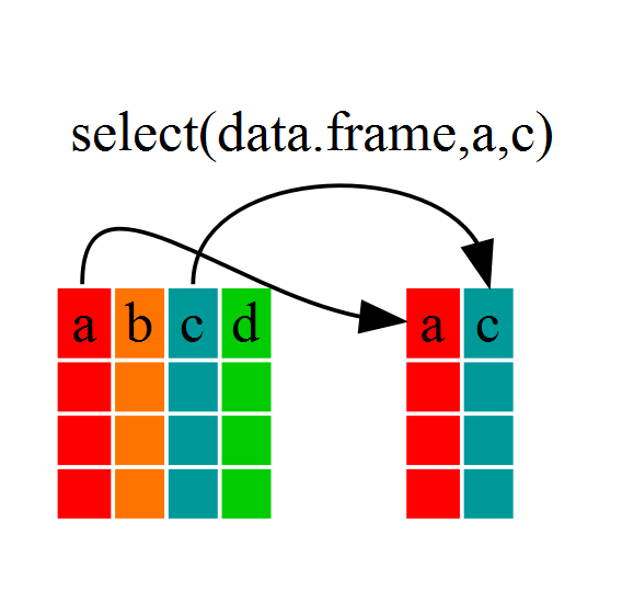
If we examine dmr_kelp we’ll see that it only contains
the year, region and kelp columns.
The Pipe
Above we used ‘normal’ grammar, but the strengths of
dplyr lie in combining several functions using pipes. Since
the pipes grammar is unlike anything we’ve seen in R before, let’s
repeat what we’ve done above using pipes.
R
dmr_kelp <- dmr |> select(year, region, kelp)
To help you understand why we wrote that in that way, let’s walk
through it step by step. First we summon the dmr data frame
and pass it on, using the pipe symbol |>, to the next
step, which is the select() function. In this case we don’t
specify which data object we use in the select() function
since in gets that from the previous pipe. Pipes can be used for more
than just dplyr functions. For example, what if we wanted
the unique region names in dmr?
R
dmr$region |> unique()
OUTPUT
[1] "York"          "Casco Bay"     "Midcoast"      "Penobscot Bay"
[5] "MDI"           "Downeast"
We can also chain pipes together. What if we wanted those unique region names sorted?
R
dmr$region |> unique() |> sort()
OUTPUT
[1] "Casco Bay"     "Downeast"      "MDI"           "Midcoast"
[5] "Penobscot Bay" "York"
To make our code more readable when we chain operations together, we often separate each step onto its own line of code.
R
dmr$region |>
  unique() |>
  sort()
This has the secondary benefit that if you’re puzzing through a particularly difficult workflow, you can write it out in comments with one step on each line, and then figure out what functions to use. Like as follows
R
#----
# Step 1: write our what you want to do

# start with regions
  # get the unique values
  # sort them


#----
# Step 2. fill in the first bit

# start with regions
dmr$region
  # get the unique values
  # sort them

#----
# Step 3. fill in the second step after looking up ??unique

# start with regions
dmr$region |>
  # get the unique values
  unique()
  # sort them

#----
# Step 4. Bring it home after googling "how to make alphabetical in R"

# start with regions
dmr$region |>
  # get the unique values
  unique() |>
  # sort them
  sort()
Callout
Fun Fact: You may have encountered pipes before in
other programming contexts. In R, a pipe symbol is |>
while in other contexts it is often | but the concept is
the same!
The |> operator is relatively new in R as part of the
base language. But, the use of pipes has been around for longer.
dplyr and many tidyverse libraries adopted the
pipe from the magrittr
library Danish data scientist Stefan Milton Bache and first released in
2014. You might see %>% in code from experienced R uses
who still use the older style pipe. There are some subtle differences
between the two, but for what we will be doing, |> will
work just fine. Also, Hadley Wickham (the original author of dplyr and
much of the tidyverse who popularized %>%) is pro-base-pipe.
Using filter()
Just as select subsets columns, filter
subsets rows using logical arguments. If we now wanted to move forward
with the above, but only with data from 2011 and kelp data, we can
combine select and filter
R
dmr_2011 <- dmr |>
  filter(year == 2011) |>
  select(year, region, kelp)
R
year_kelp_urchin_dmr <- dmr |>
                           filter(region=="Midcoast") |>
                           select(year,kelp,urchin)

nrow(year_kelp_urchin_dmr)
OUTPUT
[1] 249249 rows, as they are only the Midcoast samples
As with last time, first we pass the dmr dataframe to the
filter() function, then we pass the filtered version of the
dmr data frame to the select() function.
Note: The order of operations is very important in this
case. If we used ‘select’ first, filter would not be able to find the
variable region since we would have removed it in the previous step.
We could now do some specific operations (like calculating summary statistics) on just the Midcoast region.
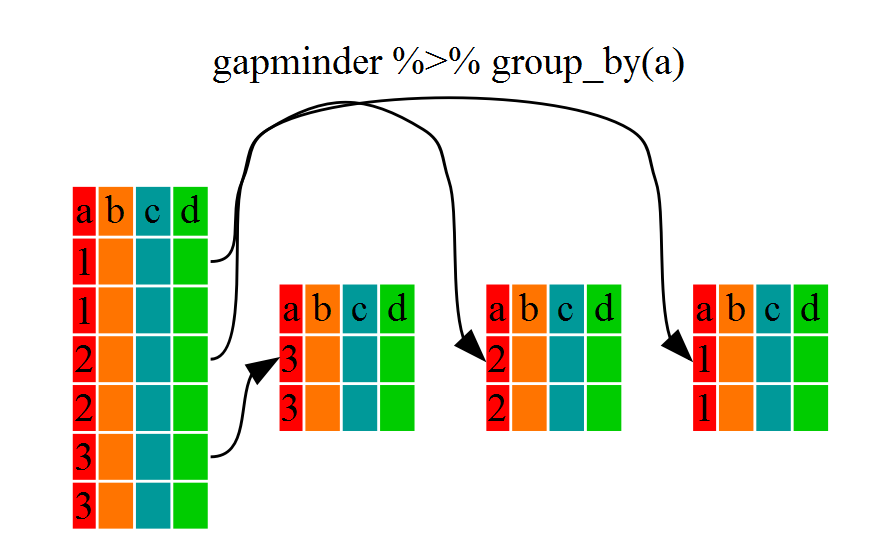
Using group_by() and summarize()
However, we were supposed to be reducing the error prone
repetitiveness of what can be done with base R! If we wanted to do
something for each region, we could take the above approach but we would
have to repeat for each region. Instead of filter(), which
will only pass observations that meet your criteria (in the above:
region==“Midcoast”), we can usegroup_by()`,
which will essentially use every unique criteria that you could have
used in filter.
R
class(dmr)
OUTPUT
[1] "data.frame"R
dmr |> group_by(region) |> class()
OUTPUT
[1] "grouped_df" "tbl_df" "tbl" "data.frame"You will notice that the structure of the dataframe where we used
group_by() (grouped_df) is not the same as the
original dmr (data.frame). A
grouped_df can be thought of as a list where
each item in the listis a data.frame which
contains only the rows that correspond to the a particular value
continent (at least in the example above).
To see this more explicitly, try str() and see the
information about groups at the end.
R
dmr |> group_by(region) |> str()
OUTPUT
gropd_df [1,478 × 15] (S3: grouped_df/tbl_df/tbl/data.frame)
 $ year         : int [1:1478] 2001 2001 2001 2001 2001 2001 2001 2001 2001 2001 ...
 $ region       : chr [1:1478] "York" "York" "York" "York" ...
 $ exposure.code: int [1:1478] 4 4 4 4 4 2 2 3 2 2 ...
 $ coastal.code : int [1:1478] 3 3 3 4 3 2 2 3 2 2 ...
 $ latitude     : num [1:1478] 43.1 43.3 43.4 43.5 43.5 ...
 $ longitude    : num [1:1478] -70.7 -70.6 -70.4 -70.3 -70.3 ...
 $ depth        : int [1:1478] 5 5 5 5 5 5 5 5 5 5 ...
 $ crust        : num [1:1478] 60 75.5 73.5 63.5 72.5 6.1 31.5 31.5 40.5 53 ...
 $ understory   : num [1:1478] 100 100 80 82 69 38.5 74 96.5 60 59.5 ...
 $ kelp         : num [1:1478] 1.9 0 18.5 0.6 63.5 92.5 59 7.7 52.5 29.2 ...
 $ urchin       : num [1:1478] 0 0 0 0 0 0 0 0 0 0 ...
 $ month        : int [1:1478] 6 6 6 6 6 6 6 6 6 6 ...
 $ day          : int [1:1478] 13 13 14 14 14 15 15 15 8 8 ...
 $ survey       : chr [1:1478] "dmr" "dmr" "dmr" "dmr" ...
 $ site         : int [1:1478] 42 47 56 61 62 66 71 70 23 22 ...
 - attr(*, "groups")= tibble [6 × 2] (S3: tbl_df/tbl/data.frame)
  ..$ region: chr [1:6] "Casco Bay" "Downeast" "MDI" "Midcoast" ...
  ..$ .rows : list<int> [1:6]
  .. ..$ : int [1:90] 6 7 8 9 10 11 12 92 93 94 ...
  .. ..$ : int [1:483] 65 66 67 68 69 70 71 72 73 74 ...
  .. ..$ : int [1:342] 44 45 46 47 48 49 50 51 52 53 ...
  .. ..$ : int [1:249] 13 14 15 16 17 18 19 20 21 22 ...
  .. ..$ : int [1:272] 32 33 34 35 36 37 38 39 40 41 ...
  .. ..$ : int [1:42] 1 2 3 4 5 90 91 170 171 172 ...
  .. ..@ ptype: int(0)
  ..- attr(*, ".drop")= logi TRUE
Using summarize()
The above was a bit on the uneventful side but
group_by() is much more exciting in conjunction with
summarize(). This will allow us to create new variable(s)
by using functions that repeat for each of the continent-specific data
frames. That is to say, using the group_by() function, we
split our original dataframe into multiple pieces, then we can run
functions (e.g. mean() or sd()) within
summarize().
R
kelp_by_region <- dmr |>
  group_by(region) |>
  summarize(mean_kelp = mean(kelp))

kelp_by_region
OUTPUT
# A tibble: 6 × 2
  region        mean_kelp
  <chr>             <dbl>
1 Casco Bay          44.1
2 Downeast           67.0
3 MDI                46.9
4 Midcoast           40.5
5 Penobscot Bay      41.1
6 York               19.4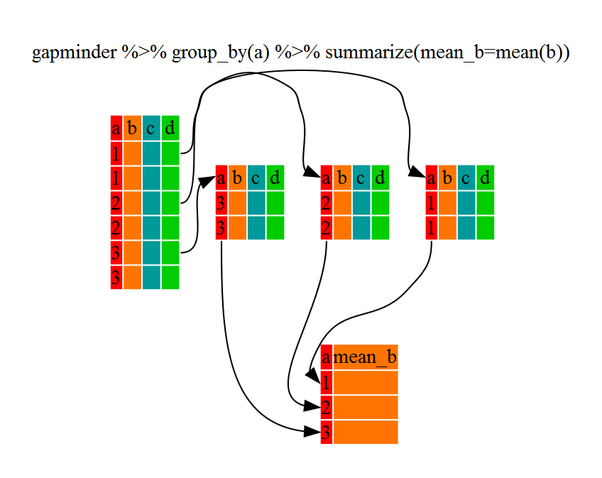
That allowed us to calculate the mean kelp % cover for each region, but it gets even better.
R
urchin_by_region <- dmr |>
   group_by(region) |>
   summarize(mean_urchins = mean(urchin))

urchin_by_region |>
   filter(mean_urchins == min(mean_urchins) | mean_urchins == max(mean_urchins))
OUTPUT
# A tibble: 2 × 2
  region        mean_urchins
  <chr>                <dbl>
1 Casco Bay           0.0767
2 Penobscot Bay       5.30
Another way to do this is to use the dplyr function
arrange(), which arranges the rows in a data frame
according to the order of one or more variables from the data frame. It
has similar syntax to other functions from the dplyr
package. You can use desc() inside arrange()
to sort in descending order.
R
urchin_by_region |>
   arrange(mean_urchins) |>
   head(1)
OUTPUT
# A tibble: 1 × 2
  region    mean_urchins
  <chr>            <dbl>
1 Casco Bay       0.0767
R
urchin_by_region |>
   arrange(desc(mean_urchins)) |>
   head(1)
OUTPUT
# A tibble: 1 × 2
  region        mean_urchins
  <chr>                <dbl>
1 Penobscot Bay         5.30
The function group_by() allows us to group by multiple
variables. Let’s group by year and region.
R
kelp_region_year <- dmr |>
  group_by(region, year) |>
  summarize(mean_kelp = mean(kelp))
OUTPUT
`summarise()` has grouped output by 'region'. You can override using the
`.groups` argument.
That is already quite powerful, but it gets even better! You’re not
limited to defining 1 new variable in summarize().
R
kelp_urchin_region_year <- dmr |>
  group_by(region, year) |>
  summarize(mean_kelp = mean(kelp),
            mean_urchin = mean(urchin),
            sd_kelp = sd(kelp),
            sd_urchin = sd(urchin))
count() and n()
A very common operation is to count the number of observations for
each group. The dplyr package comes with two related
functions that help with this.
For instance, if we wanted to check the number of countries included
in the dataset for the year 2002, we can use the count()
function. It takes the name of one or more columns that contain the
groups we are interested in, and we can optionally sort the results in
descending order by adding sort=TRUE:
R
dmr |>
    filter(year == 2002) |>
    count(region, sort = TRUE)
OUTPUT
         region  n
1      Downeast 25
2           MDI 17
3 Penobscot Bay 15
4      Midcoast 13
5     Casco Bay  8
6          York  2
If we need to use the number of observations in calculations, the
n() function is useful. For instance, if we wanted to get
the standard error of urchins per region:
R
dmr |>
    group_by(region) |>
    summarize(se_urchin = sd(urchin)/sqrt(n()))
OUTPUT
# A tibble: 6 × 2
  region        se_urchin
  <chr>             <dbl>
1 Casco Bay        0.0392
2 Downeast         0.303
3 MDI              0.388
4 Midcoast         0.227
5 Penobscot Bay    0.659
6 York             0.788
Using mutate()
We can also create new variables prior to (or even after) summarizing
information using mutate(). For example, if we wanted to
create a total_fleshy_algae column.
R
dmr |>
  mutate(total_fleshy_algae = kelp + understory)
You can also create a second new column based on the first new column
within the same call of mutate():
R
dmr |>
  mutate(total_fleshy_algae = kelp + understory,
         total_algae = total_fleshy_algae + crust)
Using mutate() and group_by()
together
In some cases, you might want to use mutate() in
conjunction with group_by() to get summarized properties
for groups, but not lose your original data. for example, let’s say we
wanted to calculate how kelp differed from average conditions within a
region each year. This is called an anomaly. In essence we want to get
the average amount of kelp in a region over time, and then calculate a
kelp_anomaly_regional where we subtract the amount of kelp
from the regional average over time. This makes it easier to separate
regional variation from variation over time.
This requires putting mutate() and
group_by() together.
R
dmr |>
  group_by(region) |>
  mutate(mean_kelp_regional = mean(kelp),
         kelp_anomaly_regional = kelp - mean_kelp_regional)
OUTPUT
# A tibble: 1,478 × 17
# Groups:   region [6]
    year region    exposure.code coastal.code latitude longitude depth crust
   <int> <chr>             <int>        <int>    <dbl>     <dbl> <int> <dbl>
 1  2001 York                  4            3     43.1     -70.7     5  60
 2  2001 York                  4            3     43.3     -70.6     5  75.5
 3  2001 York                  4            3     43.4     -70.4     5  73.5
 4  2001 York                  4            4     43.5     -70.3     5  63.5
 5  2001 York                  4            3     43.5     -70.3     5  72.5
 6  2001 Casco Bay             2            2     43.7     -70.1     5   6.1
 7  2001 Casco Bay             2            2     43.8     -70.0     5  31.5
 8  2001 Casco Bay             3            3     43.8     -69.9     5  31.5
 9  2001 Casco Bay             2            2     43.8     -69.9     5  40.5
10  2001 Casco Bay             2            2     43.8     -69.9     5  53
# ℹ 1,468 more rows
# ℹ 9 more variables: understory <dbl>, kelp <dbl>, urchin <dbl>, month <int>,
#   day <int>, survey <chr>, site <int>, mean_kelp_regional <dbl>,
#   kelp_anomaly_regional <dbl>
This worked, but, uh oh. Why is the data frame still grouped? Leaving a data frame grouped will have consequences, as any other mutate will be done by region instead of on the whole data frame. So, for example, if we wanted to then get a global anomaly, i.e., the difference between kelp and the average amount of kelp for the entire data set, we couldn’t just do another set of mutates.
Fortunately, we can resolve this with ungroup(): a
useful verb to insert any time you want to remove all grouping
structure, and are worried dplyr is not doing it for
you.
R
dmr |>
  group_by(region) |>
  mutate(mean_kelp_regional = mean(kelp),
         kelp_anomaly_regional = kelp - mean_kelp_regional) |>
  ungroup() |>
  head()
OUTPUT
# A tibble: 6 × 17
   year region    exposure.code coastal.code latitude longitude depth crust
  <int> <chr>             <int>        <int>    <dbl>     <dbl> <int> <dbl>
1  2001 York                  4            3     43.1     -70.7     5  60
2  2001 York                  4            3     43.3     -70.6     5  75.5
3  2001 York                  4            3     43.4     -70.4     5  73.5
4  2001 York                  4            4     43.5     -70.3     5  63.5
5  2001 York                  4            3     43.5     -70.3     5  72.5
6  2001 Casco Bay             2            2     43.7     -70.1     5   6.1
# ℹ 9 more variables: understory <dbl>, kelp <dbl>, urchin <dbl>, month <int>,
#   day <int>, survey <chr>, site <int>, mean_kelp_regional <dbl>,
#   kelp_anomaly_regional <dbl>
Note, it does convert your data frame into a tibble (a
“tidy” data frame), but if you really want a data frame back, you can
use as.data.frame().
Other great resources
- R for Data Science
- Data Wrangling Cheat sheet
- Introduction to dplyr
- Data wrangling with R and RStudio
Key Points
- Use the
dplyrpackage to manipulate dataframes. - Use
select()to choose variables from a dataframe. - Use
filter()to choose data based on values. - Use
group_by()andsummarize()to work with subsets of data. - Use
count()andn()to obtain the number of observations in columns. - Use
mutate()to create new variables.
Content from Introduction to Visualization
Last updated on 2024-03-12 | Edit this page
Overview
Questions
- What are the basics of creating graphics in R?
Objectives
- To be able to use ggplot2 to generate histograms and bar plots.
- To apply geometry and aesthetic layers to a ggplot plot.
- To manipulate the aesthetics of a plot using different colors and position parameters.
Let’s start by loading data to plot. For convenience, let’s make site a character.
R
library(dplyr)

dmr <- read.csv("data/dmr_kelp_urchin.csv") |>
  mutate(site = as.character(site))
Plotting our data is one of the best ways to quickly explore it and the various relationships between variables. There are three main plotting systems in R, the base plotting system, the lattice package, and the ggplot2 package. Today and tomorrow we’ll be learning about the ggplot2 package, because it is the most effective for creating publication quality graphics. In this episode, we will introduce the key features of a ggplot and make a few example plots. We will expand on these concepts and see how they apply to geospatial data types when we start working with geospatial data in the R for Raster and Vector Data lesson.
ggplot2 is built on the grammar of graphics, the idea that any plot can be expressed from the same set of components: a data set, a coordinate system, and a set of geoms (the visual representation of data points). The key to understanding ggplot2 is thinking about a figure in layers. This idea may be familiar to you if you have used image editing programs like Photoshop, Illustrator, or Inkscape. In this episode we will focus on two geoms
- histograms and bar plot. In the R for Raster and Vector Data lesson we will work with a number of other geometries and learn how to customize our plots.
Let’s start off with an example plotting the distribution of kelp %
cover in our dataset. The first thing we do is call the
ggplot function. This function lets R know that we’re
creating a new plot, and any of the arguments we give the
ggplot() function are the global options for the plot: they
apply to all layers on the plot.
We will pass in two arguments to ggplot. First, we tell
ggplot what data we want to show on our figure. For the
second argument we pass in the aes() function, which tells
ggplot how variables in the data map to aesthetic
properties of the figure. Here we will tell ggplot we want
to plot the “kelp” column of the dmr data frame on the x-axis. We don’t
need to specify a y-axis for histograms.
R
library(ggplot2)

ggplot(data = dmr,
       mapping = aes(x = kelp)) +
  geom_histogram()

By itself, the call to ggplot isn’t enough to draw a
figure:
R
ggplot(data = dmr, aes(x = kelp))
We need to tell ggplot how we want to visually represent
the data, which we do by adding a geom layer. In our example, we used
geom_histogram(), which tells ggplot we want
to visually represent the distribution of one variable (in our case
“kelp”):
R
ggplot(data = dmr, aes(x = kelp)) +
  geom_histogram()
OUTPUT
`stat_bin()` using `bins = 30`. Pick better value with `binwidth`.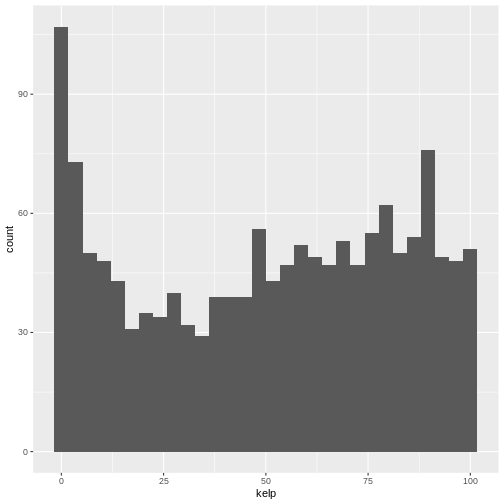
R
ggplot(data = dmr,
       mapping = aes(x = urchin)) +
 geom_histogram()
OUTPUT
`stat_bin()` using `bins = 30`. Pick better value with `binwidth`.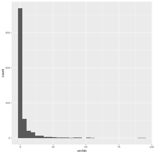
The histogram is a useful tool for visualizing the distribution of a single continuous variable. What if we want to compare the kelp cover of the regions in our dataset? We could use a bar (or column) plot.
First, let’s create a dataset with the mean % kelp for each region.
R
region_mean_kelp <- dmr |>
  group_by(region) |>
  summarize(mean_kelp = mean(kelp))
This time, we will use the geom_col() function as our
geometry. We will plot regions on the x-axis (listed in alphabetic order
by default) and mean kelp on the y-axis.
R
ggplot(data = region_mean_kelp,
       mapping = aes(x = region, y = mean_kelp)) +
  geom_col()
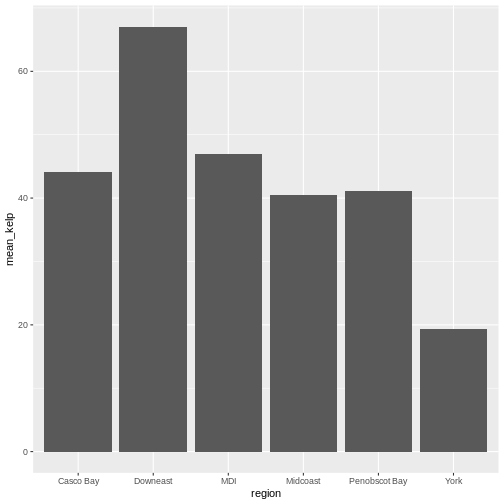
This looks okay, although perhaps you might want to display more than
just the mean values. You could try another geometry: box plots, with
geom_boxplot. Here we need the full un-summarized dataset.
You might also want to specify axis labels by using the function
labs.
R
ggplot(data = dmr,
       mapping = aes(x = region, y = kelp)) +
  geom_boxplot() +
  labs(x = "Region", y = "Percent Kelp Cover")
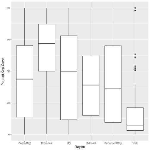
There are more sophisticated ways of modifying axis labels. We will be learning some of those methods later in this workshop.
Challenge 2: A regional subset of the data over time
Let’s combine dplyr with ggplot2 to create
a visualization of how kelp has changed by region over time. This is a
complex workflow - but a pretty typical one. We’re going to break it
down piece by piece here so you can see how we create a whole piece of
visualization starting with a large complex object.
Our goal is to create a time series plot for two regions of mean kelp.
dplyr portion - For each part of the exercise, just
keep piping to create a full workflow that will result in
casco_downeast_kelp. Check your answer after each step to
make sure it’s correct.
What are our two regions and years that we want? Let’s start by creating a data set called
casco_downeast_kelp. Filter down to just theCasco BayandDowneastregions. This is a great place to use the%in% operator for the filter. After filtering regions, filteryearto just the years 2001 - 2012. You can use some<>for this or use%in%.Next, group by both region and year (you can use a
,to separate grouping variables ingroup_by()).Summarize to get the mean value of kelp for each year/region combination.
ggplot2 portion - use
casco_downeast_kelp to plot the following.
Make a
ggplot()just like we did before with ageom_col(). But, now, set your x value to be year. Also, makefill = region. What does this show you? What happens if you add an additional argument togeom_col()so that you havegeom_col(position = position_dodge()).One of the beautiful things about
ggplot2is how we can make a few small changes and get a totally different visualization that teaches us something new. Copy and paste the plot you made in 4. Remove thegeom_col(). Now, addgeom_point()andgeom_line()in succession. Also, remove the fill aesthestic and change add incolor = regioninstead.
dplyr portion
R
casco_downeast_kelp <- dmr |>
  filter(region %in% c("Casco Bay", "Downeast")) |>
  filter(year %in% 2001:2012)

head(casco_downeast_kelp)
OUTPUT
  year    region exposure.code coastal.code latitude longitude depth crust
1 2001 Casco Bay             2            2 43.72766 -70.10721     5   6.1
2 2001 Casco Bay             2            2 43.76509 -69.96087     5  31.5
3 2001 Casco Bay             3            3 43.75199 -69.93420     5  31.5
4 2001 Casco Bay             2            2 43.78369 -69.89041     5  40.5
5 2001 Casco Bay             2            2 43.79288 -69.88675     5  53.0
6 2001 Casco Bay             1            2 43.79686 -69.88665     5  26.5
  understory  kelp urchin month day survey site
1       38.5  92.5      0     6  15    dmr   66
2       74.0  59.0      0     6  15    dmr   71
3       96.5   7.7      0     6  15    dmr   70
4       60.0  52.5      0     6   8    dmr   23
5       59.5  29.2      0     6   8    dmr   22
6       15.0 100.0      0     6   8    dmr   21
R
casco_downeast_kelp <- dmr |>
  filter(region %in% c("Casco Bay", "Downeast")) |>
  filter(year %in% 2001:2012) |>
  group_by(year, region)

head(casco_downeast_kelp)
OUTPUT
# A tibble: 6 × 15
# Groups:   year, region [1]
   year region    exposure.code coastal.code latitude longitude depth crust
  <int> <chr>             <int>        <int>    <dbl>     <dbl> <int> <dbl>
1  2001 Casco Bay             2            2     43.7     -70.1     5   6.1
2  2001 Casco Bay             2            2     43.8     -70.0     5  31.5
3  2001 Casco Bay             3            3     43.8     -69.9     5  31.5
4  2001 Casco Bay             2            2     43.8     -69.9     5  40.5
5  2001 Casco Bay             2            2     43.8     -69.9     5  53
6  2001 Casco Bay             1            2     43.8     -69.9     5  26.5
# ℹ 7 more variables: understory <dbl>, kelp <dbl>, urchin <dbl>, month <int>,
#   day <int>, survey <chr>, site <chr>
R
casco_downeast_kelp <- dmr |>
  filter(region %in% c("Casco Bay", "Downeast")) |>
  filter(year %in% 2001:2012) |>
  group_by(year, region) |>
  summarize(mean_kelp = mean(kelp))
OUTPUT
`summarise()` has grouped output by 'year'. You can override using the
`.groups` argument.
R
head(casco_downeast_kelp)
OUTPUT
# A tibble: 6 × 3
# Groups:   year [3]
   year region    mean_kelp
  <int> <chr>         <dbl>
1  2001 Casco Bay      48.8
2  2001 Downeast       74.3
3  2002 Casco Bay      56.7
4  2002 Downeast       78.8
5  2003 Casco Bay      58.7
6  2003 Downeast       89.2
ggplot2 portion
R
ggplot(data = casco_downeast_kelp,
       mapping = aes(x = year, y = mean_kelp, fill = region)) +
  geom_col()
R
ggplot(data = casco_downeast_kelp,
       mapping = aes(x = year, y = mean_kelp, fill = region)) +
  geom_col(position = position_dodge())
R
ggplot(data = casco_downeast_kelp,
       mapping = aes(x = year, y = mean_kelp, color = region)) +
  geom_point() +
  geom_line()
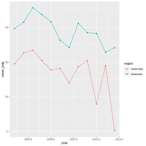
The examples given here are just the start of creating complex and beautiful graphics with R. In a later lesson we will go into much more depth, including:
- plotting geospatial specific data types
- adjusting the color scheme of our plots
- setting and formatting plot titles, subtitles, and axis labels
- creating multi-panel plots
- creating point (scatter) and line plots
- layering datasets to create multi-layered plots
- creating and customizing a plot legend
- and much more!
The examples we’ve worked through in this episode should give you the building blocks for working with the more complex graphic types and customizations we will be working with in that lesson.
Content from Writing Data
Last updated on 2024-03-12 | Edit this page
Overview
Questions
- How can I save plots and data created in R?
Objectives
- To be able to write out plots and data from R.
If you haven’t already, you should create directories to save cleaned data and figures.
R
dir.create("cleaned-data")
dir.create("figures")
Saving plots
You can save a plot from within RStudio using the ‘Export’ button in the ‘Plot’ window. This will give you the option of saving as a .pdf or as .png, .jpg or other image formats.
Sometimes you will want to save plots without creating them in the
‘Plot’ window first. Perhaps you want to make a pdf document with
multiple pages: each one a different plot, for example. Or perhaps
you’re looping through multiple subsets of a file, plotting data from
each subset, and you want to save each plot. In this case you can use a
more flexible approach. The pdf() function creates a new
pdf device. You can control the size and resolution using the arguments
to this function.
R
pdf("figures/Distribution-of-kelp.pdf", width=12, height=4)

ggplot(data = dmr, aes(x = kelp)) +
  geom_histogram()

# You then have to make sure to turn off the pdf device!
dev.off()
Open up this document and have a look.
R
pdf("figures/Distribution-of-kelp-urchins.pdf", width = 12, height = 4)

ggplot(data = dmr,
       mapping = aes(x = kelp)) +
geom_histogram()

ggplot(data = dmr,
       mapping = aes(x = urchin)) +
  geom_histogram()

dev.off()
The commands jpeg, png, etc. are used
similarly to produce documents in different formats. You can also use
ggsave() to save whatever your last plot was. For example,
let’s say we made a neat plot using geom_point() (a
scatterplot) to show the relationship between kelp and urchins colored
by region. We want to save it as a jpeg. ggsave() will
dynamically figure out your filetype from the file name.
R
ggplot(dmr,
       aes(x = urchin, y = kelp,
           color = region)) +
  geom_point()
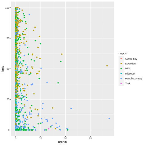
R
ggsave("figures/kelp_urchin.jpg")
OUTPUT
Saving 7 x 7 in imageWriting data
At some point, you’ll also want to write out data from R.
We can use the write.csv function for this, which is
very similar to read.csv from before.
Let’s create a data-cleaning script, for this analysis, we only want to focus on the data for Downeast:
R
downeast_subset <- dmr |>
  filter(region == "Downeast")

write.csv(downeast_subset,
  file="cleaned-data/dmr_downeast.csv"
)
Let’s open the file to make sure it contains the data we expect.
Navigate to your cleaned-data directory and double-click
the file name. It will open using your computer’s default for opening
files with a .csv extension. To open in a specific
application, right click and select the application. Using a spreadsheet
program (like Excel) to open this file shows us that we do have properly
formatted data including only the data points from Downeast. However,
there are row numbers associated with the data that are not useful to us
(they refer to the row numbers from the gapminder data frame).
Let’s look at the help file to work out how to change this behaviour.
R
?write.csv
By default R will write out the row and column names when writing data to a file. To over write this behavior, we can do the following:
R
write.csv(
  downeast_subset,
  file = "cleaned-data/dmr_downeast.csv",
  row.names=FALSE
)
R
dmr_after_2012 <- filter(dmr, year > 2012)

write.csv(dmr_after_2012,
  file = "cleaned-data/dmr_after_2012.csv",
  row.names = FALSE)