Introduction to Visualization
Last updated on 2024-03-12 | Edit this page
Overview
Questions
- What are the basics of creating graphics in R?
Objectives
- To be able to use ggplot2 to generate histograms and bar plots.
- To apply geometry and aesthetic layers to a ggplot plot.
- To manipulate the aesthetics of a plot using different colors and position parameters.
Let’s start by loading data to plot. For convenience, let’s make site a character.
R
library(dplyr)

dmr <- read.csv("data/dmr_kelp_urchin.csv") |>
  mutate(site = as.character(site))
Plotting our data is one of the best ways to quickly explore it and the various relationships between variables. There are three main plotting systems in R, the base plotting system, the lattice package, and the ggplot2 package. Today and tomorrow we’ll be learning about the ggplot2 package, because it is the most effective for creating publication quality graphics. In this episode, we will introduce the key features of a ggplot and make a few example plots. We will expand on these concepts and see how they apply to geospatial data types when we start working with geospatial data in the R for Raster and Vector Data lesson.
ggplot2 is built on the grammar of graphics, the idea that any plot can be expressed from the same set of components: a data set, a coordinate system, and a set of geoms (the visual representation of data points). The key to understanding ggplot2 is thinking about a figure in layers. This idea may be familiar to you if you have used image editing programs like Photoshop, Illustrator, or Inkscape. In this episode we will focus on two geoms
- histograms and bar plot. In the R for Raster and Vector Data lesson we will work with a number of other geometries and learn how to customize our plots.
Let’s start off with an example plotting the distribution of kelp %
cover in our dataset. The first thing we do is call the
ggplot function. This function lets R know that we’re
creating a new plot, and any of the arguments we give the
ggplot() function are the global options for the plot: they
apply to all layers on the plot.
We will pass in two arguments to ggplot. First, we tell
ggplot what data we want to show on our figure. For the
second argument we pass in the aes() function, which tells
ggplot how variables in the data map to aesthetic
properties of the figure. Here we will tell ggplot we want
to plot the “kelp” column of the dmr data frame on the x-axis. We don’t
need to specify a y-axis for histograms.
R
library(ggplot2)

ggplot(data = dmr,
       mapping = aes(x = kelp)) +
  geom_histogram()

By itself, the call to ggplot isn’t enough to draw a
figure:
R
ggplot(data = dmr, aes(x = kelp))
We need to tell ggplot how we want to visually represent
the data, which we do by adding a geom layer. In our example, we used
geom_histogram(), which tells ggplot we want
to visually represent the distribution of one variable (in our case
“kelp”):
R
ggplot(data = dmr, aes(x = kelp)) +
  geom_histogram()
OUTPUT
`stat_bin()` using `bins = 30`. Pick better value with `binwidth`.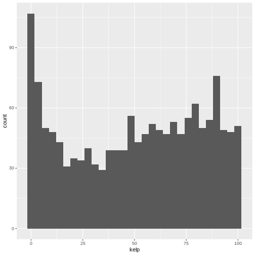
R
ggplot(data = dmr,
       mapping = aes(x = urchin)) +
 geom_histogram()
OUTPUT
`stat_bin()` using `bins = 30`. Pick better value with `binwidth`.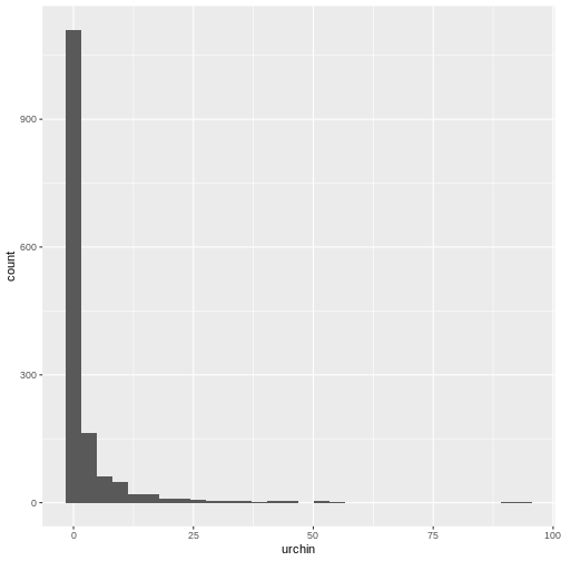
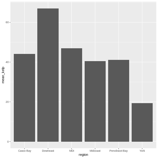
The histogram is a useful tool for visualizing the distribution of a single continuous variable. What if we want to compare the kelp cover of the regions in our dataset? We could use a bar (or column) plot.
First, let’s create a dataset with the mean % kelp for each region.
R
region_mean_kelp <- dmr |>
  group_by(region) |>
  summarize(mean_kelp = mean(kelp))
This time, we will use the geom_col() function as our
geometry. We will plot regions on the x-axis (listed in alphabetic order
by default) and mean kelp on the y-axis.
R
ggplot(data = region_mean_kelp,
       mapping = aes(x = region, y = mean_kelp)) +
  geom_col()
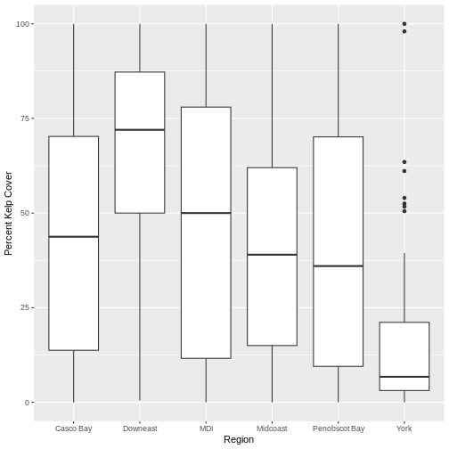
This looks okay, although perhaps you might want to display more than
just the mean values. You could try another geometry: box plots, with
geom_boxplot. Here we need the full un-summarized dataset.
You might also want to specify axis labels by using the function
labs.
R
ggplot(data = dmr,
       mapping = aes(x = region, y = kelp)) +
  geom_boxplot() +
  labs(x = "Region", y = "Percent Kelp Cover")
There are more sophisticated ways of modifying axis labels. We will be learning some of those methods later in this workshop.
Challenge 2: A regional subset of the data over time
Let’s combine dplyr with ggplot2 to create
a visualization of how kelp has changed by region over time. This is a
complex workflow - but a pretty typical one. We’re going to break it
down piece by piece here so you can see how we create a whole piece of
visualization starting with a large complex object.
Our goal is to create a time series plot for two regions of mean kelp.
dplyr portion - For each part of the exercise, just
keep piping to create a full workflow that will result in
casco_downeast_kelp. Check your answer after each step to
make sure it’s correct.
What are our two regions and years that we want? Let’s start by creating a data set called
casco_downeast_kelp. Filter down to just theCasco BayandDowneastregions. This is a great place to use the%in% operator for the filter. After filtering regions, filteryearto just the years 2001 - 2012. You can use some<>for this or use%in%.Next, group by both region and year (you can use a
,to separate grouping variables ingroup_by()).Summarize to get the mean value of kelp for each year/region combination.
ggplot2 portion - use
casco_downeast_kelp to plot the following.
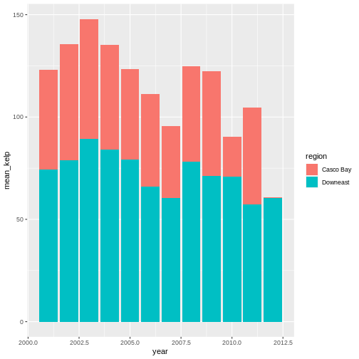
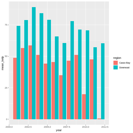
Make a
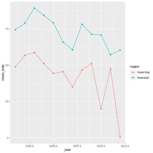
ggplot()just like we did before with ageom_col(). But, now, set your x value to be year. Also, makefill = region. What does this show you? What happens if you add an additional argument togeom_col()so that you havegeom_col(position = position_dodge()).One of the beautiful things about
ggplot2is how we can make a few small changes and get a totally different visualization that teaches us something new. Copy and paste the plot you made in 4. Remove thegeom_col(). Now, addgeom_point()andgeom_line()in succession. Also, remove the fill aesthestic and change add incolor = regioninstead.
dplyr portion
R
casco_downeast_kelp <- dmr |>
  filter(region %in% c("Casco Bay", "Downeast")) |>
  filter(year %in% 2001:2012)

head(casco_downeast_kelp)
OUTPUT
  year    region exposure.code coastal.code latitude longitude depth crust
1 2001 Casco Bay             2            2 43.72766 -70.10721     5   6.1
2 2001 Casco Bay             2            2 43.76509 -69.96087     5  31.5
3 2001 Casco Bay             3            3 43.75199 -69.93420     5  31.5
4 2001 Casco Bay             2            2 43.78369 -69.89041     5  40.5
5 2001 Casco Bay             2            2 43.79288 -69.88675     5  53.0
6 2001 Casco Bay             1            2 43.79686 -69.88665     5  26.5
  understory  kelp urchin month day survey site
1       38.5  92.5      0     6  15    dmr   66
2       74.0  59.0      0     6  15    dmr   71
3       96.5   7.7      0     6  15    dmr   70
4       60.0  52.5      0     6   8    dmr   23
5       59.5  29.2      0     6   8    dmr   22
6       15.0 100.0      0     6   8    dmr   21
R
casco_downeast_kelp <- dmr |>
  filter(region %in% c("Casco Bay", "Downeast")) |>
  filter(year %in% 2001:2012) |>
  group_by(year, region)

head(casco_downeast_kelp)
OUTPUT
# A tibble: 6 × 15
# Groups:   year, region [1]
   year region    exposure.code coastal.code latitude longitude depth crust
  <int> <chr>             <int>        <int>    <dbl>     <dbl> <int> <dbl>
1  2001 Casco Bay             2            2     43.7     -70.1     5   6.1
2  2001 Casco Bay             2            2     43.8     -70.0     5  31.5
3  2001 Casco Bay             3            3     43.8     -69.9     5  31.5
4  2001 Casco Bay             2            2     43.8     -69.9     5  40.5
5  2001 Casco Bay             2            2     43.8     -69.9     5  53
6  2001 Casco Bay             1            2     43.8     -69.9     5  26.5
# ℹ 7 more variables: understory <dbl>, kelp <dbl>, urchin <dbl>, month <int>,
#   day <int>, survey <chr>, site <chr>
R
casco_downeast_kelp <- dmr |>
  filter(region %in% c("Casco Bay", "Downeast")) |>
  filter(year %in% 2001:2012) |>
  group_by(year, region) |>
  summarize(mean_kelp = mean(kelp))
OUTPUT
`summarise()` has grouped output by 'year'. You can override using the
`.groups` argument.
R
head(casco_downeast_kelp)
OUTPUT
# A tibble: 6 × 3
# Groups:   year [3]
   year region    mean_kelp
  <int> <chr>         <dbl>
1  2001 Casco Bay      48.8
2  2001 Downeast       74.3
3  2002 Casco Bay      56.7
4  2002 Downeast       78.8
5  2003 Casco Bay      58.7
6  2003 Downeast       89.2
ggplot2 portion
R
ggplot(data = casco_downeast_kelp,
       mapping = aes(x = year, y = mean_kelp, fill = region)) +
  geom_col()
R
ggplot(data = casco_downeast_kelp,
       mapping = aes(x = year, y = mean_kelp, fill = region)) +
  geom_col(position = position_dodge())
R
ggplot(data = casco_downeast_kelp,
       mapping = aes(x = year, y = mean_kelp, color = region)) +
  geom_point() +
  geom_line()
The examples given here are just the start of creating complex and beautiful graphics with R. In a later lesson we will go into much more depth, including:
- plotting geospatial specific data types
- adjusting the color scheme of our plots
- setting and formatting plot titles, subtitles, and axis labels
- creating multi-panel plots
- creating point (scatter) and line plots
- layering datasets to create multi-layered plots
- creating and customizing a plot legend
- and much more!
The examples we’ve worked through in this episode should give you the building blocks for working with the more complex graphic types and customizations we will be working with in that lesson.