Writing Data

Overview

Questions

• How can I save plots and data created in R?

Objectives

• To be able to write out plots and data from R.

If you haven’t already, you should create directories to save cleaned data and figures.

R

dir.create("cleaned-data")
dir.create("figures")

Saving plots

---

You can save a plot from within RStudio using the ‘Export’ button in the ‘Plot’ window. This will give you the option of saving as a .pdf or as .png, .jpg or other image formats.

Sometimes you will want to save plots without creating them in the ‘Plot’ window first. Perhaps you want to make a pdf document with multiple pages: each one a different plot, for example. Or perhaps you’re looping through multiple subsets of a file, plotting data from each subset, and you want to save each plot. In this case you can use a more flexible approach. The pdf() function creates a new pdf device. You can control the size and resolution using the arguments to this function.

R

pdf("figures/Distribution-of-kelp.pdf", width=12, height=4)

ggplot(data = dmr, aes(x = kelp)) +   
  geom_histogram()

# You then have to make sure to turn off the pdf device!
dev.off()

Open up this document and have a look.

Challenge 1

Rewrite your ‘pdf’ command to print a second page in the pdf, showing the histogram of urchins in the data.

Solution to challenge 1

R

pdf("figures/Distribution-of-kelp-urchins.pdf", width = 12, height = 4)

ggplot(data = dmr, 
       mapping = aes(x = kelp)) + 
geom_histogram()

ggplot(data = dmr, 
       mapping = aes(x = urchin)) +
  geom_histogram()

dev.off()

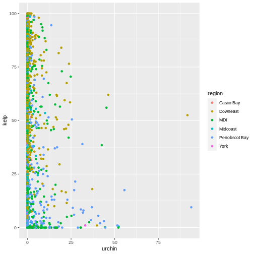
The commands jpeg, png, etc. are used similarly to produce documents in different formats. You can also use ggsave() to save whatever your last plot was. For example, let’s say we made a neat plot using geom_point() (a scatterplot) to show the relationship between kelp and urchins colored by region. We want to save it as a jpeg. ggsave() will dynamically figure out your filetype from the file name.

R

ggplot(dmr,
       aes(x = urchin, y = kelp,
           color = region)) +
  geom_point()

R

ggsave("figures/kelp_urchin.jpg")

OUTPUT

Saving 7 x 7 in image

Writing data

---

At some point, you’ll also want to write out data from R.

We can use the write.csv function for this, which is very similar to read.csv from before.

Let’s create a data-cleaning script, for this analysis, we only want to focus on the data for Downeast:

R

downeast_subset <- dmr |>
  filter(region == "Downeast")

write.csv(downeast_subset,
  file="cleaned-data/dmr_downeast.csv"
)

Let’s open the file to make sure it contains the data we expect. Navigate to your cleaned-data directory and double-click the file name. It will open using your computer’s default for opening files with a .csv extension. To open in a specific application, right click and select the application. Using a spreadsheet program (like Excel) to open this file shows us that we do have properly formatted data including only the data points from Downeast. However, there are row numbers associated with the data that are not useful to us (they refer to the row numbers from the gapminder data frame).

Let’s look at the help file to work out how to change this behaviour.

R

?write.csv

By default R will write out the row and column names when writing data to a file. To over write this behavior, we can do the following:

R

write.csv(
  downeast_subset,
  file = "cleaned-data/dmr_downeast.csv",
  row.names=FALSE
)

Challenge 2

Subset the dmr data to include only data points collected since 2012. Write out the new subset to a file in the cleaned-data/ directory.

Solution to challenge 2

R

dmr_after_2012 <- filter(dmr, year > 2012)

write.csv(dmr_after_2012,
  file = "cleaned-data/dmr_after_2012.csv",
  row.names = FALSE)

Key Points

• Save plots using ggsave() or pdf() combined with dev.off().
• Use write.csv to save tabular data.