Spatial Selection
Last updated on 2024-02-20 | Edit this page
Overview
Questions
- How can I use interactive maps as an input select?
- How can I make my spatial apps more interactive?
Objectives
- Use leaflet in Shiny.
- Demonstrate the basic building blocks of a Shiny app.
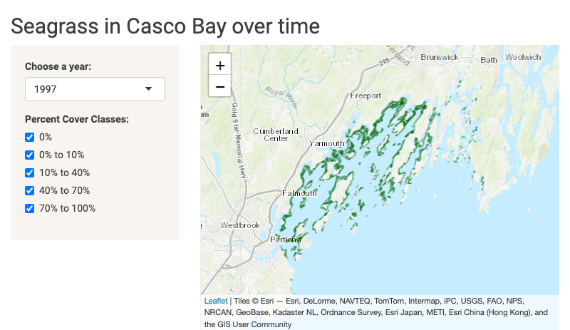
Our App So Far
We’ve been doing great work on our app to look at seagrass beds in Casco Bay. Let’s summarize where we are so far, although we will remove the histogram for the moment.
R
# 1. Preamble
library(shiny)
library(shinythemes)
library(sf)
library(dplyr)
library(ggplot2)

seagrass_casco <- readRDS("data/joined_seagrass_cover.Rds")

# 2. Define a User Interface
ui <- fluidPage(
  title = "Seagrass in Casco App",
  theme = shinytheme("sandstone"),

 titlePanel("Seagrass in Casco Bay over time"),

 sidebarLayout(

   # sidebar
   sidebarPanel(
     selectInput(
       inputId = "year",
       label = "Choose a year:",
       choices = unique(seagrass_casco$year) |> sort(),
       selected = unique(seagrass_casco$year) |> min() #to get the earliest year
       ),

     checkboxGroupInput(
       inputId = "cover",
       label = "Percent Cover Classes:",
       choices = unique(seagrass_casco$cover_pct) |> sort(),
       selected =  unique(seagrass_casco$cover_pct) |> sort()
     ),
   ),

   # main
   mainPanel(
     plotOutput("map"),
   )
 )
)

# 3. define a server
server <- function(input, output) {

  # our map block
  output$map <- renderPlot({

    dat <- seagrass_casco |>
      filter(year %in% input$year) |>
      filter(cover_pct %in% input$cover)

    ggplot() +
      geom_sf(data = dat,
              linewidth = 1.5,
              color = "darkgreen")

  })


}
This is great, BUT, it could be improved greatly in two ways. First, why not have our map me more interactive - a leaflet map! Second, let’s actually add some color to our beds by cover.
Leaflet in Shiny Apps
Forunately, leaflet provides functions to work inside of
a Shiny app just like a plot. There is a leafletOutput()
and renderLeaflet() function. We can simply change the
plotOutput("map") in our UI to
leafletOutput("map"). Then, we can modify the server.
R
# 3. define a server
server <- function(input, output) {

  # our map block
  output$map <- renderLeaflet({

    dat <- seagrass_casco |>
      filter(year %in% input$year) |>
      filter(cover_pct %in% input$cover)

    leaflet() |>
      addProviderTiles("Esri.WorldTopoMap") |>
      addPolygons(data = dat,
                  color = "darkgreen",
                  weight = 1.5)

  })


}
Making a Reactive Leaflet Map
While this is awesome, as we can change our map easily, one frustration you might have noticed is that every time you change an input, the map resets its field of view. That’s because every time you change an input, Shiny re-runs the output, and it remakes the map from scratch. Not ideal.
Instead, we can use leafletProxy() to update a map. To
use leafletProxy(), we first create a map output with only
the parts of the map that will not respond to inputs. We can then treat
our map as a reactive object insofar as we will use
observe() to make changes are made. In our case, as our
selectors change the data used for the map, we will make the data a
reactive, and then use the reactive data for the observe()
statement.
Within our observe(), we will use
leafletProxy() with the argument mapId to
refer to the leaflet output - in this case "map". To it, we
will also have to add clearShapes() in order to plot only
what we are selecting. Otherwise, layers will be added on layers will be
added on layers will be….
Let’s look at our new server with the reactive, a static map (that includes bounds, as otherwise we’d start at a global scale), and our observe statement.
R
server <- function(input, output) {

  ## A reactive for data
  dat <- reactive({
    seagrass_casco |>
      filter(year %in% input$year) |>
      filter(cover_pct %in% input$cover)
  })

  ## An initial map with **only** elements that one' change
  output$map <- renderLeaflet({
    #we will need some initial bounds
    b <- st_bbox(seagrass_casco) |> as.numeric()

    leaflet() |>
      addProviderTiles("Esri.WorldTopoMap") |>
      fitBounds(b[1], b[2], b[3], b[4])

  })

  ## An observe statement to update the map
  observe({
    # here we use leafletProxy()
    leafletProxy(mapId = "map", data = dat()) |>
      clearShapes() |>
      addPolygons(
                  color = "darkgreen",
                  weight = 1.5)


  })

}
This now works as advertised!
Using Elements of a Leaflet Map as Input
As we have constructed a beautiful visualization of seagrass beds in Casco Bay, maybe we want to know more about each of those individual beds. We know that each polygon has a lot of information associated with it. For example.
R
seagrass_casco[1,]
Let’s say, for each bed, we want to be able to click on it and see
the information in that row of data. With leaflet maps, we can actually
do this without Shiny to some degree with the popup
argument. So, for example, we can make a map of 1997 with popups. We
will use paste() to make the text understandable.
R
seagrass_casco |>
  filter(year == 1997) |>
  leaflet() |>
  addTiles() |>
  addPolygons(popup = ~paste("Acres: ", acres))
We can do this for more than just acres. We can also use the
label argument to make this information popup when we just
mouse over the polygon.
This might be all you need! But, what if we want to do
something with the selected polygon data. Let’s say, for example,
we wanted to output the row of data the polygon came from. To do that,
we need to give each polygon an individual ID. Let’s add
bed_id column to the data that is just the row number. We
can put this in our preamble.
R
seagrass_casco <- seagrass_casco |>
  mutate(bed_id = 1:n())
To add this to our app, we can now add a layerId
argument to our polygon. We will use ~ to say that we are
going to evaluate one of the variables from
R
  ## An observe statement to update the map
  observe({
    # here we use leafletProxy()
    leafletProxy(mapId = "map", data = dat()) |>
      clearShapes() |>
      addPolygons(
                  color = "darkgreen",
                  weight = 1.5,
                  layerId = ~bed_id)


  })
So, now that we have layer IDs, how can we make them respond to
clicking on polygons? The answer is that interacting with
leaflet maps does trigger an input. We interact with maps
in two ways. One is with the whole map. The other is with just pieces.
Let’s focus on the later. The input triggered is
input$MAPID_OBJCATEGORY_EVENTNAMEwhere MAPID is the input ID of the map (here map),
OBJCATEGORY is a category descriptor of an object in a leaflet map. See
here for a
list of valid ones - what concerns us is shape and
marker. And last, EVENTNAME which is either
click, mouseover or mouseout.
So, for a click on a polygon, we’d be looking at
input$map_shape_clickTo show what this outputs, let’s insert two pieces into our code.
First, in the UI, add verbatimTextOutput("layer_click") and
to the server add
R
  output$layer_click <- renderText({
    capture.output(print(input$map_shape_click))
  })
From this, when we run the ap and click on a bed, we get output like this
$id [1] 3824 $.nonce [1] 0.8434182 $lat [1] 43.79836 $lng [1] -70.10101 OH! A list! With an ID which is the bed_id. We can do
something with that!
For the moment, let’s just show the hectares of the bed clicked on. We can do that by filtering to the bed ID and outputting text.
R
  output$layer_click <- renderText({
    one_row <- seagrass_casco |> filter(bed_id == input$map_shape_click$id)

    paste("This bed is", one_row$hectares, "hectares")
  })
Ew. What’s that initial output? To fix output when there is no click,
we need to return something for the NULL case.
R
  output$layer_click <- renderText({
    if(is.null(input$map_shape_click)) return("")

    one_row <- seagrass_casco |> filter(bed_id == input$map_shape_click)

    paste("This bed is", one_row$hectares, "hectares")
  })
Selecting With Your Map in Leaflet
What if, instead of what we’ve clicked on, we want information about
the area we are looking within? We have two options. The first is to use
the map itself as our selector. Like the
input$MAPID_OBJCATEGORY_EVENTNAME above, there is also just
an input$MAPID_EVENTNAME for the whole map.
These events include click which will return the
lat and lng of where you click,
center which does the same for where your map is centered,
zoom which will return your zoom level, and
bounds which will return the corner coordinates of your
map. north, east, south, and
west.
Below our text output in the UI, let’s add a
plotOutput("hectare_hist") and in our UI add a function
that crops our reactive dat() to the bounds of our
input$bounds. We can st_crop() with an
st_bbox() made from the bounds.
R
  # show the bed hectares
  output$hectare_hist <- renderPlot({
    # our crop box
    #xmin ymin xmax ymax
    crop_box <- st_bbox(c(xmin = input$map_bounds$west,
                        ymin = input$map_bounds$south,
                        xmax = input$map_bounds$east,
                        ymax = input$map_bounds$north),
                        crs = 4326)

    hist_data <- st_crop(dat(), crop_box)

    ggplot(data = hist_data, aes(x = hectares)) +
      geom_histogram(bins = 30)
  })
Selecting with a Draw Box
If you want to get fancy and use a drawing box instead, we need to
use something extra - the leaflet.extras
package. Lots of people have written Javascript extensions to Leaflet.
This package and leaflet.extras2
have tried to capture some of these into R. For our purposes, we need to
add an addDrawToolbar() to our map in the server.
R
  ## An initial map with **only** elements that one' change
  output$map <- renderLeaflet({
    #we will need some initial bounds
    b <- st_bbox(seagrass_casco) |> as.numeric()

    leaflet() |>
      addProviderTiles("Esri.WorldTopoMap") |>
      fitBounds(b[1], b[2], b[3], b[4]) |>
      addDrawToolbar(position = "topright",
                     editOptions =
                       editToolbarOptions(edit = FALSE))

  })
Note the editOptions. That’s just so we can have a trash
can to get rid of selectors once we are done.
This toolbar now produces the ability to draw shapes on a map and return information from them. Again, as above, using one of these will generate an input.
input$MAPID_draw_EVENTNAMEThere are a wide variety of EVENTNAME possibilities which are listed
here.
For our purposes, as we want to make a new histogram every time a square
is drawn, we want input$map_draw_new_feature which triggers
anytime a new feature is drawn.
What does this input return? Unfortunately, what it returns is a list
in the geojson format. Fortunately, we can use the geojsonsf
package to turn it into an sf object, and then crop as before to make
the histogram. Let’s change our histogram in our server to
R
  # show the bed hectares
  output$hectare_hist <- renderPlot({
    # good behavior
    if(is.null(input$map_draw_new_feature)) return(NA)

    # our crop box
    selected_shape <- input$map_draw_new_feature

    crop_sf <-
      geojsonsf::geojson_sf(jsonify::to_json(selected_shape, unbox = T))

    hist_data <- st_crop(dat(), crop_sf)

    ggplot(data = hist_data, aes(x = hectares)) +
      geom_histogram(bins = 30)
  })
And now take it for a spin!
Callout
That was a lot! For your future reference, here is the final code for the app by the end of this lesson. It’s a mid-sized app, but, a really nice one that accomplishes some very fancy tasks! Well done!
If you want to see a working version of it, try this link.
R
# 1. Preamble
library(shiny)
library(shinythemes)
library(sf)
library(dplyr)
library(ggplot2)
library(leaflet)
library(leaflet.extras)

seagrass_casco <- readRDS("data/joined_seagrass_cover.Rds")

seagrass_casco <- seagrass_casco |>
  mutate(bed_id = 1:n())


# 2. Define a User Interface
ui <- fluidPage(
  title = "Seagrass in Casco App",
  theme = shinytheme("sandstone"),

  titlePanel("Seagrass in Casco Bay over time"),

  sidebarLayout(

    # sidebar
    sidebarPanel(
      selectInput(
        inputId = "year",
        label = "Choose a year:",
        choices = unique(seagrass_casco$year) |> sort(),
        selected = unique(seagrass_casco$year) |> min() #to get the earliest year
      ),

      checkboxGroupInput(
        inputId = "cover",
        label = "Percent Cover Classes:",
        choices = unique(seagrass_casco$cover_pct) |> sort(),
        selected =  unique(seagrass_casco$cover_pct) |> sort()
      ),
    ),

    # main
    mainPanel(
      leafletOutput("map"),
      verbatimTextOutput("layer_click"),
      plotOutput("hectare_hist")
    )
  )
)

# 3. define a server
server <- function(input, output) {

  ## A reactive for data
  dat <- reactive({
    seagrass_casco |>
      filter(year %in% input$year) |>
      filter(cover_pct %in% input$cover)
  })

  ## An initial map with **only** elements that one' change
  output$map <- renderLeaflet({
    #we will need some initial bounds
    b <- st_bbox(seagrass_casco) |> as.numeric()

    leaflet() |>
      addProviderTiles("Esri.WorldTopoMap") |>
      fitBounds(b[1], b[2], b[3], b[4]) |>
      addDrawToolbar(position = "topright",
                     editOptions =
                       editToolbarOptions(edit = FALSE))

  })

  ## An observe statement to update the map
  observe({
    # here we use leafletProxy()
    leafletProxy(mapId = "map", data = dat()) |>
      clearShapes() |>
      addPolygons(
        color = "darkgreen",
        weight = 1.5,
        layerId = ~bed_id)


  })

  output$layer_click <- renderText({
    if(is.null(input$map_shape_click)) return("")

    one_row <- seagrass_casco |> filter(bed_id == input$map_shape_click$id)

    paste("This bed is", one_row$hectares, "hectares")
  })

  # show the bed hectares
  output$hectare_hist <- renderPlot({
    # good behavior
    if(is.null(input$map_draw_new_feature)) return(NA)

    # our crop box
    selected_shape <- input$map_draw_new_feature

    crop_sf <-
      geojsonsf::geojson_sf(jsonify::to_json(selected_shape, unbox = T))

    hist_data <- st_crop(dat(), crop_sf)

    ggplot(data = hist_data, aes(x = hectares)) +
      geom_histogram(bins = 30)
  })

}