Content from Introduction to Shiny
Last updated on 2024-02-20 | Edit this page
Overview
Questions
- What is a Shiny App?
Objectives
- Explain what a Shiny app can do.
- Demonstrate the basic building blocks of a Shiny app.
Introduction to Shiny
As many of us work in R, we often want to make our work viewable to others in a broad audience. There are tools, such as Quarto that allow you to generate rich static reports that can be re-made every time your data updates (worth digging into another time!). They do not let other people play with the data and visualizations you are working on without their digging into the guts of R.
The answer is the creation of web applications. Shiny is a package that allows one to create web applications swiftly to explore and interact with data. At their bare minimum, they allow for some simple selection of subsets of data and re-visualizations. At their most complex… well, chekc out some of the submissions to the annual R Shiny Competition.
 Shiny in a Nutshell
from Dean Attali
Shiny in a Nutshell
from Dean Attali
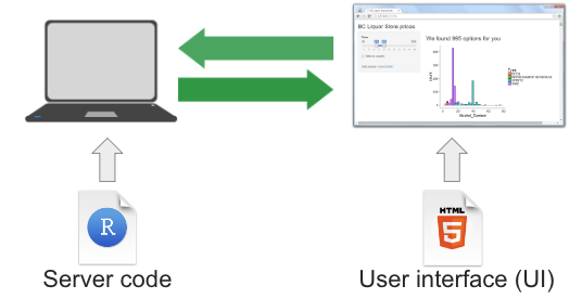
In a nutshell, we write Shiny apps in R code. Those apps are then hosted on a server that is running an instance of a Shiny Server. Note, we will use a public Shiny server for this lesson, shinyapps.io. A user goes to the URL of a shiny site. The server processes the R code and delivers a user interface.
Discussion: Some example Shiny Sites
Here are a few Shiny websites. Take some time to explore them. What do you like about them? What do you not like about them? What possibilities do you see for your own work?
Posit’s shiny gallery.
Sea Surface Temperature from Buoys in the Gulf of Maine
Map of sites sampled by Maine DMR and the Rasher and Steneck labs for kelp and urchins.
Change in algal compsition from 1980-2014 at Appledore Island
Subtidal videos of kelp surves in Salem Sound
Creating a Shiny App
Let’s start by creating a new project called
shiny-geospatial. Within that project, create a folder
called data and download FIXME into that folder. Now, create a new
script. Call it app.R. Save it in the same director as your
.Rproj file.
Callout
While you can put a Shiny app into any file you like, once you use it
with a Shiny server, and you want to go to
http://myshinyserver.com/my_cool_app/ to run your app, the
server will only recognize one of two configurations.
The app is in a file called
app.Rin your top level directory. This file will have your entire app.The app is split between
ui.Randserver.R- which have those two pieces respectively.
Otherwise, nothing will load. You can create other R files with apps
in them to test out different things, but, they will not be recognized
by a server. This is not to say you won’t put pieces of your app in
different R files - we will talk about this later - but you will call
them within your app.R file using
source().
Note, you could have also created a Shiny project from Rstudio. But, this would initialize with a pre-built Shiny app in it. Which is fun to play with, but, can be confusing to then re-edit later.
The Anatomy of a Shiny App
A shiny app consists of four distinct parts. Here they all are, laid out. This app will actually run, although it will produce a blank app. Here’s the whole piece laid out. We will look at each one in turn.
R
# 1. Preamble
library(shiny)

# 2. Define a User Interface
ui <- fluidPage()

# 3. define a server
server <- function(input, output) {}

# 4. Call shinyApp() to run your app
shinyApp(ui = ui, server = server)
First, the preamble. This is code to run at the top
of the app (including loading the Shiny package) to prepare objects,
color palettes, or other things that you do not need dynamically created
or recreated later. You can even write this in another R script - say,
create_objects.R and then run them in the preamble like
so:
R
source("create_objects.R")
Second, the User Interface.
R
# 2. Define a User Interface
ui <- fluidPage()
Here, we create an object called ui for later use. We
are using the fluidPage() function. What does that do? The
helpfile tells us this is a function that creates a fluid page layout,
and we can add a title, theme, and more. What does that mean? Let’s find
out.
R
ui
We see that fluidPage() has generated some HTML code.
This is the core of Shiny - functions that generate code to be
interpreted by a web browser.
Note, because of the (), we can see that this is a
function. Shiny user interfaces are built by a series of nested
functions, each one generating more and more HTML code, nested by order
of how the functions are written.
Third we have the server:
R
# 3. define a server
server <- function(input, output) {}
This is, at the moment, just an empty function definition with two
arguments. What are those arguments? Where do they come from? Where are
they going? In Shiny, these are both defined by the environment. As we
will see input is a list modified by the ui.
And output is also a list that will be modified by the
server.
The final section is the call to Shiny. It runs the app
itself. So, you can call this to run the app. Note that the ui and
server are inputs to the arguments ui and
server. This means that, if you wanted, you could have
named them something else, but, the community seems to have coalesced
around using these object names.
R
# 4. Call shinyApp() to run your app
shinyApp(ui = ui, server = server)
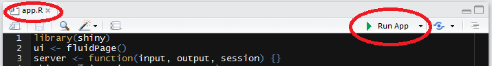
Do you need to run this line of code every time? In Rstudio, no. As long as it sees this is a shiny app, there will be some options to run the app in your window
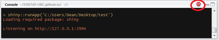
Which will also start a server. You can stop the server at any time by either hitting Ctrl-C in the console, or, clicking the Stop button in RStudio.
Content from The Basics of a User Interface
Last updated on 2024-02-20 | Edit this page
Overview
Questions
- How do we build a User Interface?
Objectives
Learn how to add elements to a UI.
Discover the different layouts and lewks you can create with Shiny.
How do we make things show up in our user interface? The R Shiny ecosystem provides a dynamic layout ecosystem about which much has been written. It’s also constantly being updated and extended by other packages. Here we will begin to add code to our blank app to begin to build something useful to explore data regarding seagrass beds in Casco Bay.
Adding Text to the UI
Starting with our blank app, what happens if we add a little text to
the fluidPage()
R
# 1. Preamble
library(shiny)

# 2. Define a User Interface
ui <- fluidPage(
  "An app about seagrass.",
  "Different Years"
)

# 3. define a server
server <- function(input, output) {}

# 4. Call shinyApp() to run your app
shinyApp(ui = ui, server = server)

FYI, from this point forward, we will just show the parts of the app we are working on, rather than the whole thing.
So, the above is nice. But, 1) It’s just small text and 2) the webpage didn’t have a title. How can we make it look better?
First, note that
R
fluidPage(
  "An app about seagrass.",
  "Different Years"
)
An app about seagrass. Different Years
outputs HTML code again. Within fluidPage() we can
either add HTML code directly with the HTML() function. Or,
if you don’t know/want to learn HTML, Shiny comes with a number of
functions that will generate valid HTML code. You can look these up with
?tags or with names(tags). Note, the later
will show even more possible functions, but for many of them, you have
to use tags$*().
For example:
R
fluidPage(
  h1("An app about seagrass."),
  br(),
  h3("Different Years")
)
An app about seagrass.
Different Years
Generates one big header, a line break, and a smaller header. Let’s add this to our UI and see what it looks like.
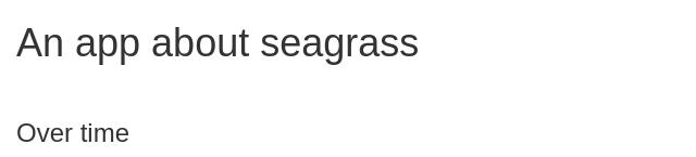
R
ui <- fluidPage(
  h1("An app about seagrass"),
  br(),
  h3("Over time")
)
 If we
want our app to have a title, we can give it one as well.
If we
want our app to have a title, we can give it one as well.
R
ui <- fluidPage(
  title = "Seagrass in Casco App",
  h1("An app about seagrass"),
  br(),
  h3("Over time")
)
Note how every piece is separated by a comma.
Explore names(tags) and use different functions to
create a small website you like. You can look at ?tags to
get information about some of them, or just play with
tags$*() to format things in different ways. If a tag can
take other arguments, you can supply them as arguments to the function.
If you have no idea what any of this might mean, check out this html reference.
For example
R
ui <- fluidPage(
  title = "Seagrass in Casco App",
  tags$strong("I am strong"),
  br(),
  tags$blockquote("Here I quoteth from the finest."),
  br(),
  a("Maine Historical Eeelgrass Viewer", href = "https://maine.maps.arcgis.com/apps/MapSeries/index.html?appid=ac2f7b3d29b34268a230a060d6b78b25")
)
Adding a Theme
To see the different pieces of the layout as we move forward, we’re
also going to add a theme. A theme isn’t necessary, but can often make
things shine. The bslib package proves a dynamic tool to
make themes. However, to do so quickly, we recomment shinythemes. Let’s add
the sandstone theme.
R
library(shinythemes)

ui <- fluidPage(
  title = "Seagrass in Casco App",
  theme = shinytheme("sandstone"),

  h1("An app about seagrass"),
  br(),
  h3("Over time")
)
We don’t see it making a huge difference yet, but notice how the font changes. Themes are another great example of an item that one can find many resouces on, but it’s a rabbit hole you can become lost inside of.
Adding Layouts to the UI
Rather than hand-coding all of the HTML in a page, Shiny provides a number of functions that will create dynamic interfaces and blocks of HTML code for you. Check out Posit’s guide to layouts for a fairly comprehensive guide or this chapter from Mastering Shiny. For our purposes, we will use the classic sidebar layout. Let’s start by taking our raw text and making a title panel.
R
ui <- fluidPage(
  title = "Seagrass in Casco App",
  theme = shinytheme("sandstone"),

 titlePanel("Seagrass in Casco Bay over time")
)
To that, we will use a classic sidebarLayout(). Within a
sidebarLayout() we also need to add a
sidebarPanel() and mainPanel, as otherwise the
layout would just be a blank box.
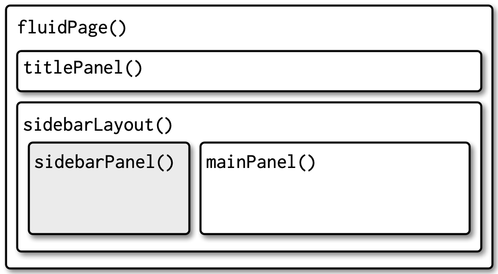 The nesting of a
sidebar layout from [Mastering Shiny](https://mastering-shiny.org/action-layout.html
The nesting of a
sidebar layout from [Mastering Shiny](https://mastering-shiny.org/action-layout.html
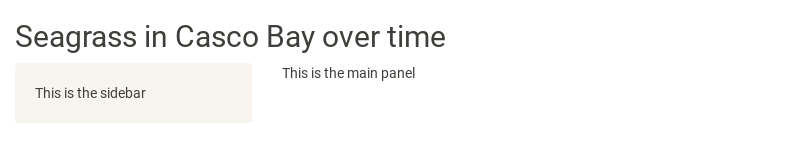
R
ui <- fluidPage(
  title = "Seagrass in Casco App",
  theme = shinytheme("sandstone"),

 titlePanel("Seagrass in Casco Bay over time"),

 sidebarLayout(
   sidebarPanel("This is the sidebar"),
   mainPanel("This is the main panel")
 )
)
You might have noticed that there is an inherent column/row layout
here. Fluid pages are structured using fluid rows and columns nested
within fluid rows. There are 12 units of width across a fluid row. Using
fluidRow() and column() make a UI with 3 rows,
3 columns in row 1, 2 in row 2, and 1 in row 3. All dividing the row
equally. Put text into them to see the results.
Note, you might have to stretch your viewing window to see it.
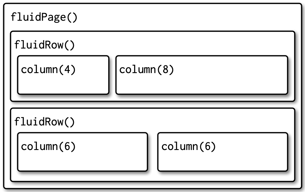 A multirow layout from Mastering
Shiny
A multirow layout from Mastering
Shiny
R
ui <- fluidPage(
  fluidRow(
    column(4,
      "1,1"
    ),
    column(4,
      "1,2"
    ),
    column(4,
      "1,3"
    )
  ),
  fluidRow(
    column(6,
     "2,1"
    ),
    column(6,
      "2,2"
    )
  ),
  fluidRow(
    column(12,
      "3,1"
    )
  )
)
Content from Inputs and Outputs
Last updated on 2024-02-20 | Edit this page
ERROR
Error: package or namespace load failed for 'units' in dyn.load(file, DLLpath = DLLpath, ...):
 unable to load shared object '/home/runner/.local/share/renv/cache/v5/R-4.3/x86_64-pc-linux-gnu/units/0.8-5/119d19da480e873f72241ff6962ffd83/units/libs/units.so':
  libudunits2.so.0: cannot open shared object file: No such file or directory
ERROR
Error: package or namespace load failed for 'sf' in dyn.load(file, DLLpath = DLLpath, ...):
 unable to load shared object '/home/runner/.local/share/renv/cache/v5/R-4.3/x86_64-pc-linux-gnu/units/0.8-5/119d19da480e873f72241ff6962ffd83/units/libs/units.so':
  libudunits2.so.0: cannot open shared object file: No such file or directory
Overview
Questions
- How do we let users query the data?
- How do we change the data to let the app respond to the user?
Objectives
- Show how to add inputs and spaces for outputs to an app UI.
- Demonstrate server logic to create custom reactive outputs.
Adding Data to Our App Thus Far
So far, we have created an app with a basic layout
R
# 1. Preamble
library(shiny)
library(shinythemes)

# 2. Define a User Interface
ui <- fluidPage(
  title = "Seagrass in Casco App",
  theme = shinytheme("sandstone"),

 titlePanel("Seagrass in Casco Bay over time"),

 sidebarLayout(
   sidebarPanel("This is the sidebar"),
   mainPanel("This is the main panel")
 )
)

# 3. define a server
server <- function(input, output) {}

# 4. Call shinyApp() to run your app
shinyApp(ui = ui, server = server)
We don’t create apps to be static and bare, however. We want this app
to explore data from Maine
DEP surveys of Seagrass Beds through time. To make this easier, here
we provide a saved sf object that is merged seagrass data
through time. Note, this is not a raw shapefile, but rather the result
of some post-processing of the data layers provided by the Maine
GeoLibrary.
You
can download the data here. Note how small .Rds files
are. This was generated with saveRds() which can save out
any R object.
Challenge
To the preamble of your all, load the
sfpackage, thedplyrpackage, and load the data usingreadRDS(). It works just likemy_dat <- read.csv("data/my_data.csv). Let’s call this dataseagrass_casco.Explore the data a bit. What are the columns? What is the projection? What years are here? How many beds are there per year? What are the potential percent cover classes?
R
library(sf)
ERROR
Error: package or namespace load failed for 'sf' in dyn.load(file, DLLpath = DLLpath, ...):
 unable to load shared object '/home/runner/.local/share/renv/cache/v5/R-4.3/x86_64-pc-linux-gnu/units/0.8-5/119d19da480e873f72241ff6962ffd83/units/libs/units.so':
  libudunits2.so.0: cannot open shared object file: No such file or directory
R
library(dplyr)

seagrass_casco <- readRDS("data/joined_seagrass_cover.Rds")
R
#what is here
str(seagrass_casco)
OUTPUT
Classes 'sf' and 'data.frame':	4946 obs. of  7 variables:
 $ year     : num  2022 2022 2022 2022 2022 ...
 $ acres    : num  0.0446 0.0608 2.5622 0.7182 0.0182 ...
 $ hectares : num  0.01803 0.02459 1.03688 0.29063 0.00735 ...
 $ cover    : int  1 3 3 3 3 3 1 1 3 4 ...
 $ cover_pct: chr  "0% to 10%" "40% to 70%" "40% to 70%" "40% to 70%" ...
 $ year97   : int  NA NA NA NA NA NA NA NA NA NA ...
 $ geometry :List of 4946
  ..$ :List of 1
  .. ..$ : num [1:55, 1:2] -70.2 -70.2 -70.2 -70.2 -70.2 ...
  .. ..- attr(*, "class")= chr [1:3] "XY" "POLYGON" "sfg"
  ..$ :List of 1
  .. ..$ : num [1:39, 1:2] -70.2 -70.2 -70.2 -70.2 -70.2 ...
  .. ..- attr(*, "class")= chr [1:3] "XY" "POLYGON" "sfg"
  ..$ :List of 1
  .. ..$ : num [1:145, 1:2] -70.2 -70.2 -70.2 -70.2 -70.2 ...
  .. ..- attr(*, "class")= chr [1:3] "XY" "POLYGON" "sfg"
  ..$ :List of 1
  .. ..$ : num [1:68, 1:2] -70.2 -70.2 -70.2 -70.2 -70.2 ...
  .. ..- attr(*, "class")= chr [1:3] "XY" "POLYGON" "sfg"
  ..$ :List of 1
  .. ..$ : num [1:18, 1:2] -70.2 -70.2 -70.2 -70.2 -70.2 ...
  .. ..- attr(*, "class")= chr [1:3] "XY" "POLYGON" "sfg"
  ..$ :List of 1
  .. ..$ : num [1:38, 1:2] -70.2 -70.2 -70.2 -70.2 -70.2 ...
  .. ..- attr(*, "class")= chr [1:3] "XY" "POLYGON" "sfg"
  ..$ :List of 1
  .. ..$ : num [1:37, 1:2] -70.2 -70.2 -70.2 -70.2 -70.2 ...
  .. ..- attr(*, "class")= chr [1:3] "XY" "POLYGON" "sfg"
  ..$ :List of 1
  .. ..$ : num [1:60, 1:2] -70.2 -70.2 -70.2 -70.2 -70.2 ...
  .. ..- attr(*, "class")= chr [1:3] "XY" "POLYGON" "sfg"
  ..$ :List of 1
  .. ..$ : num [1:21, 1:2] -70.2 -70.2 -70.2 -70.2 -70.2 ...
  .. ..- attr(*, "class")= chr [1:3] "XY" "POLYGON" "sfg"
  ..$ :List of 1
  .. ..$ : num [1:103, 1:2] -70.2 -70.2 -70.2 -70.2 -70.2 ...
  .. ..- attr(*, "class")= chr [1:3] "XY" "POLYGON" "sfg"
  ..$ :List of 1
  .. ..$ : num [1:48, 1:2] -70.2 -70.2 -70.2 -70.2 -70.2 ...
  .. ..- attr(*, "class")= chr [1:3] "XY" "POLYGON" "sfg"
  ..$ :List of 1
  .. ..$ : num [1:32, 1:2] -70.2 -70.2 -70.2 -70.2 -70.2 ...
  .. ..- attr(*, "class")= chr [1:3] "XY" "POLYGON" "sfg"
  ..$ :List of 1
  .. ..$ : num [1:64, 1:2] -70.2 -70.2 -70.2 -70.2 -70.2 ...
  .. ..- attr(*, "class")= chr [1:3] "XY" "POLYGON" "sfg"
  ..$ :List of 1
  .. ..$ : num [1:78, 1:2] -70.2 -70.2 -70.2 -70.2 -70.2 ...
  .. ..- attr(*, "class")= chr [1:3] "XY" "POLYGON" "sfg"
  ..$ :List of 1
  .. ..$ : num [1:47, 1:2] -70.2 -70.2 -70.2 -70.2 -70.2 ...
  .. ..- attr(*, "class")= chr [1:3] "XY" "POLYGON" "sfg"
  ..$ :List of 1
  .. ..$ : num [1:29, 1:2] -70.2 -70.2 -70.2 -70.2 -70.2 ...
  .. ..- attr(*, "class")= chr [1:3] "XY" "POLYGON" "sfg"
  ..$ :List of 1
  .. ..$ : num [1:54, 1:2] -70.2 -70.2 -70.2 -70.2 -70.2 ...
  .. ..- attr(*, "class")= chr [1:3] "XY" "POLYGON" "sfg"
  ..$ :List of 1
  .. ..$ : num [1:22, 1:2] -70.2 -70.2 -70.2 -70.2 -70.2 ...
  .. ..- attr(*, "class")= chr [1:3] "XY" "POLYGON" "sfg"
  ..$ :List of 1
  .. ..$ : num [1:36, 1:2] -70.2 -70.2 -70.2 -70.2 -70.2 ...
  .. ..- attr(*, "class")= chr [1:3] "XY" "POLYGON" "sfg"
  ..$ :List of 1
  .. ..$ : num [1:258, 1:2] -70.2 -70.2 -70.2 -70.2 -70.2 ...
  .. ..- attr(*, "class")= chr [1:3] "XY" "POLYGON" "sfg"
  ..$ :List of 1
  .. ..$ : num [1:29, 1:2] -70.2 -70.2 -70.2 -70.2 -70.2 ...
  .. ..- attr(*, "class")= chr [1:3] "XY" "POLYGON" "sfg"
  ..$ :List of 1
  .. ..$ : num [1:11, 1:2] -70.2 -70.2 -70.2 -70.2 -70.2 ...
  .. ..- attr(*, "class")= chr [1:3] "XY" "POLYGON" "sfg"
  ..$ :List of 1
  .. ..$ : num [1:22, 1:2] -70.2 -70.2 -70.2 -70.2 -70.2 ...
  .. ..- attr(*, "class")= chr [1:3] "XY" "POLYGON" "sfg"
  ..$ :List of 1
  .. ..$ : num [1:11, 1:2] -70.2 -70.2 -70.2 -70.2 -70.2 ...
  .. ..- attr(*, "class")= chr [1:3] "XY" "POLYGON" "sfg"
  ..$ :List of 1
  .. ..$ : num [1:28, 1:2] -70.2 -70.2 -70.2 -70.2 -70.2 ...
  .. ..- attr(*, "class")= chr [1:3] "XY" "POLYGON" "sfg"
  ..$ :List of 1
  .. ..$ : num [1:431, 1:2] -70.2 -70.2 -70.2 -70.2 -70.2 ...
  .. ..- attr(*, "class")= chr [1:3] "XY" "POLYGON" "sfg"
  ..$ :List of 1
  .. ..$ : num [1:116, 1:2] -70.2 -70.2 -70.2 -70.2 -70.2 ...
  .. ..- attr(*, "class")= chr [1:3] "XY" "POLYGON" "sfg"
  ..$ :List of 1
  .. ..$ : num [1:203, 1:2] -70.2 -70.2 -70.2 -70.2 -70.2 ...
  .. ..- attr(*, "class")= chr [1:3] "XY" "POLYGON" "sfg"
  ..$ :List of 1
  .. ..$ : num [1:47, 1:2] -70.2 -70.2 -70.2 -70.2 -70.2 ...
  .. ..- attr(*, "class")= chr [1:3] "XY" "POLYGON" "sfg"
  ..$ :List of 1
  .. ..$ : num [1:358, 1:2] -70.2 -70.2 -70.2 -70.2 -70.2 ...
  .. ..- attr(*, "class")= chr [1:3] "XY" "POLYGON" "sfg"
  ..$ :List of 1
  .. ..$ : num [1:58, 1:2] -70.2 -70.2 -70.2 -70.2 -70.2 ...
  .. ..- attr(*, "class")= chr [1:3] "XY" "POLYGON" "sfg"
  ..$ :List of 1
  .. ..$ : num [1:186, 1:2] -70.2 -70.2 -70.2 -70.2 -70.2 ...
  .. ..- attr(*, "class")= chr [1:3] "XY" "POLYGON" "sfg"
  ..$ :List of 3
  .. ..$ : num [1:159, 1:2] -70.2 -70.2 -70.2 -70.2 -70.2 ...
  .. ..$ : num [1:23, 1:2] -70.2 -70.2 -70.2 -70.2 -70.2 ...
  .. ..$ : num [1:40, 1:2] -70.2 -70.2 -70.2 -70.2 -70.2 ...
  .. ..- attr(*, "class")= chr [1:3] "XY" "POLYGON" "sfg"
  ..$ :List of 3
  .. ..$ : num [1:184, 1:2] -70.2 -70.2 -70.2 -70.2 -70.2 ...
  .. ..$ : num [1:16, 1:2] -70.2 -70.2 -70.2 -70.2 -70.2 ...
  .. ..$ : num [1:11, 1:2] -70.2 -70.2 -70.2 -70.2 -70.2 ...
  .. ..- attr(*, "class")= chr [1:3] "XY" "POLYGON" "sfg"
  ..$ :List of 1
  .. ..$ : num [1:35, 1:2] -70.2 -70.2 -70.2 -70.2 -70.2 ...
  .. ..- attr(*, "class")= chr [1:3] "XY" "POLYGON" "sfg"
  ..$ :List of 1
  .. ..$ : num [1:141, 1:2] -70.2 -70.2 -70.2 -70.2 -70.2 ...
  .. ..- attr(*, "class")= chr [1:3] "XY" "POLYGON" "sfg"
  ..$ :List of 1
  .. ..$ : num [1:38, 1:2] -70.2 -70.2 -70.2 -70.2 -70.2 ...
  .. ..- attr(*, "class")= chr [1:3] "XY" "POLYGON" "sfg"
  ..$ :List of 1
  .. ..$ : num [1:68, 1:2] -70 -70 -70 -70 -70 ...
  .. ..- attr(*, "class")= chr [1:3] "XY" "POLYGON" "sfg"
  ..$ :List of 1
  .. ..$ : num [1:34, 1:2] -70 -70 -70 -70 -70 ...
  .. ..- attr(*, "class")= chr [1:3] "XY" "POLYGON" "sfg"
  ..$ :List of 1
  .. ..$ : num [1:51, 1:2] -70 -70 -70 -70 -70 ...
  .. ..- attr(*, "class")= chr [1:3] "XY" "POLYGON" "sfg"
  ..$ :List of 1
  .. ..$ : num [1:29, 1:2] -70 -70 -70 -70 -70 ...
  .. ..- attr(*, "class")= chr [1:3] "XY" "POLYGON" "sfg"
  ..$ :List of 1
  .. ..$ : num [1:29, 1:2] -70 -70 -70 -70 -70 ...
  .. ..- attr(*, "class")= chr [1:3] "XY" "POLYGON" "sfg"
  ..$ :List of 1
  .. ..$ : num [1:28, 1:2] -70 -70 -70 -70 -70 ...
  .. ..- attr(*, "class")= chr [1:3] "XY" "POLYGON" "sfg"
  ..$ :List of 1
  .. ..$ : num [1:57, 1:2] -70 -70 -70 -70 -70 ...
  .. ..- attr(*, "class")= chr [1:3] "XY" "POLYGON" "sfg"
  ..$ :List of 1
  .. ..$ : num [1:28, 1:2] -70 -70 -70 -70 -70 ...
  .. ..- attr(*, "class")= chr [1:3] "XY" "POLYGON" "sfg"
  ..$ :List of 1
  .. ..$ : num [1:36, 1:2] -70 -70 -70 -70 -70 ...
  .. ..- attr(*, "class")= chr [1:3] "XY" "POLYGON" "sfg"
  ..$ :List of 1
  .. ..$ : num [1:40, 1:2] -70.1 -70.1 -70.1 -70.1 -70.1 ...
  .. ..- attr(*, "class")= chr [1:3] "XY" "POLYGON" "sfg"
  ..$ :List of 1
  .. ..$ : num [1:39, 1:2] -70.1 -70.1 -70.1 -70.1 -70.1 ...
  .. ..- attr(*, "class")= chr [1:3] "XY" "POLYGON" "sfg"
  ..$ :List of 1
  .. ..$ : num [1:36, 1:2] -70.1 -70.1 -70.1 -70.1 -70.1 ...
  .. ..- attr(*, "class")= chr [1:3] "XY" "POLYGON" "sfg"
  ..$ :List of 2
  .. ..$ : num [1:82, 1:2] -70.1 -70.1 -70.1 -70.1 -70.1 ...
  .. ..$ : num [1:46, 1:2] -70.1 -70.1 -70.1 -70.1 -70.1 ...
  .. ..- attr(*, "class")= chr [1:3] "XY" "POLYGON" "sfg"
  ..$ :List of 1
  .. ..$ : num [1:26, 1:2] -70.1 -70.1 -70.1 -70.1 -70.1 ...
  .. ..- attr(*, "class")= chr [1:3] "XY" "POLYGON" "sfg"
  ..$ :List of 1
  .. ..$ : num [1:19, 1:2] -70.1 -70.1 -70.1 -70.1 -70.1 ...
  .. ..- attr(*, "class")= chr [1:3] "XY" "POLYGON" "sfg"
  ..$ :List of 1
  .. ..$ : num [1:36, 1:2] -70.1 -70.1 -70.1 -70.1 -70.1 ...
  .. ..- attr(*, "class")= chr [1:3] "XY" "POLYGON" "sfg"
  ..$ :List of 1
  .. ..$ : num [1:56, 1:2] -70.1 -70.1 -70.1 -70.1 -70.1 ...
  .. ..- attr(*, "class")= chr [1:3] "XY" "POLYGON" "sfg"
  ..$ :List of 1
  .. ..$ : num [1:24, 1:2] -70.1 -70.1 -70.1 -70.1 -70.1 ...
  .. ..- attr(*, "class")= chr [1:3] "XY" "POLYGON" "sfg"
  ..$ :List of 1
  .. ..$ : num [1:91, 1:2] -70.1 -70.1 -70.1 -70.1 -70.1 ...
  .. ..- attr(*, "class")= chr [1:3] "XY" "POLYGON" "sfg"
  ..$ :List of 1
  .. ..$ : num [1:65, 1:2] -70.1 -70.1 -70.1 -70.1 -70.1 ...
  .. ..- attr(*, "class")= chr [1:3] "XY" "POLYGON" "sfg"
  ..$ :List of 1
  .. ..$ : num [1:24, 1:2] -70.1 -70.1 -70.1 -70.1 -70.1 ...
  .. ..- attr(*, "class")= chr [1:3] "XY" "POLYGON" "sfg"
  ..$ :List of 1
  .. ..$ : num [1:16, 1:2] -70.1 -70.1 -70.1 -70.1 -70.1 ...
  .. ..- attr(*, "class")= chr [1:3] "XY" "POLYGON" "sfg"
  ..$ :List of 1
  .. ..$ : num [1:71, 1:2] -70.1 -70.1 -70.1 -70.1 -70.1 ...
  .. ..- attr(*, "class")= chr [1:3] "XY" "POLYGON" "sfg"
  ..$ :List of 1
  .. ..$ : num [1:76, 1:2] -70.1 -70.1 -70.1 -70.1 -70.1 ...
  .. ..- attr(*, "class")= chr [1:3] "XY" "POLYGON" "sfg"
  ..$ :List of 1
  .. ..$ : num [1:67, 1:2] -70.1 -70.1 -70.1 -70.1 -70.1 ...
  .. ..- attr(*, "class")= chr [1:3] "XY" "POLYGON" "sfg"
  ..$ :List of 1
  .. ..$ : num [1:97, 1:2] -70.1 -70.1 -70.1 -70.1 -70.1 ...
  .. ..- attr(*, "class")= chr [1:3] "XY" "POLYGON" "sfg"
  ..$ :List of 1
  .. ..$ : num [1:40, 1:2] -70.1 -70.1 -70.1 -70.1 -70.1 ...
  .. ..- attr(*, "class")= chr [1:3] "XY" "POLYGON" "sfg"
  ..$ :List of 1
  .. ..$ : num [1:142, 1:2] -70.1 -70.1 -70.1 -70.1 -70.1 ...
  .. ..- attr(*, "class")= chr [1:3] "XY" "POLYGON" "sfg"
  ..$ :List of 1
  .. ..$ : num [1:29, 1:2] -70.1 -70.1 -70.1 -70.1 -70.1 ...
  .. ..- attr(*, "class")= chr [1:3] "XY" "POLYGON" "sfg"
  ..$ :List of 1
  .. ..$ : num [1:35, 1:2] -70.2 -70.2 -70.2 -70.2 -70.2 ...
  .. ..- attr(*, "class")= chr [1:3] "XY" "POLYGON" "sfg"
  ..$ :List of 1
  .. ..$ : num [1:41, 1:2] -70.2 -70.2 -70.2 -70.2 -70.2 ...
  .. ..- attr(*, "class")= chr [1:3] "XY" "POLYGON" "sfg"
  ..$ :List of 1
  .. ..$ : num [1:54, 1:2] -70.2 -70.2 -70.2 -70.2 -70.2 ...
  .. ..- attr(*, "class")= chr [1:3] "XY" "POLYGON" "sfg"
  ..$ :List of 1
  .. ..$ : num [1:15, 1:2] -70.2 -70.2 -70.2 -70.2 -70.2 ...
  .. ..- attr(*, "class")= chr [1:3] "XY" "POLYGON" "sfg"
  ..$ :List of 1
  .. ..$ : num [1:44, 1:2] -70.2 -70.2 -70.2 -70.2 -70.2 ...
  .. ..- attr(*, "class")= chr [1:3] "XY" "POLYGON" "sfg"
  ..$ :List of 1
  .. ..$ : num [1:71, 1:2] -70.2 -70.2 -70.2 -70.2 -70.2 ...
  .. ..- attr(*, "class")= chr [1:3] "XY" "POLYGON" "sfg"
  ..$ :List of 1
  .. ..$ : num [1:40, 1:2] -70.2 -70.2 -70.2 -70.2 -70.2 ...
  .. ..- attr(*, "class")= chr [1:3] "XY" "POLYGON" "sfg"
  ..$ :List of 1
  .. ..$ : num [1:10, 1:2] -70.2 -70.2 -70.2 -70.2 -70.2 ...
  .. ..- attr(*, "class")= chr [1:3] "XY" "POLYGON" "sfg"
  ..$ :List of 1
  .. ..$ : num [1:31, 1:2] -70.2 -70.2 -70.2 -70.2 -70.2 ...
  .. ..- attr(*, "class")= chr [1:3] "XY" "POLYGON" "sfg"
  ..$ :List of 1
  .. ..$ : num [1:26, 1:2] -70.2 -70.2 -70.2 -70.2 -70.2 ...
  .. ..- attr(*, "class")= chr [1:3] "XY" "POLYGON" "sfg"
  ..$ :List of 1
  .. ..$ : num [1:38, 1:2] -70.2 -70.2 -70.2 -70.2 -70.2 ...
  .. ..- attr(*, "class")= chr [1:3] "XY" "POLYGON" "sfg"
  ..$ :List of 1
  .. ..$ : num [1:67, 1:2] -70.1 -70.1 -70.1 -70.1 -70.1 ...
  .. ..- attr(*, "class")= chr [1:3] "XY" "POLYGON" "sfg"
  ..$ :List of 1
  .. ..$ : num [1:73, 1:2] -70.1 -70.1 -70.1 -70.1 -70.1 ...
  .. ..- attr(*, "class")= chr [1:3] "XY" "POLYGON" "sfg"
  ..$ :List of 1
  .. ..$ : num [1:263, 1:2] -70.1 -70.1 -70.1 -70.1 -70.1 ...
  .. ..- attr(*, "class")= chr [1:3] "XY" "POLYGON" "sfg"
  ..$ :List of 1
  .. ..$ : num [1:21, 1:2] -70.2 -70.2 -70.2 -70.2 -70.2 ...
  .. ..- attr(*, "class")= chr [1:3] "XY" "POLYGON" "sfg"
  ..$ :List of 1
  .. ..$ : num [1:299, 1:2] -70.2 -70.2 -70.2 -70.2 -70.2 ...
  .. ..- attr(*, "class")= chr [1:3] "XY" "POLYGON" "sfg"
  ..$ :List of 1
  .. ..$ : num [1:50, 1:2] -70.2 -70.2 -70.2 -70.2 -70.2 ...
  .. ..- attr(*, "class")= chr [1:3] "XY" "POLYGON" "sfg"
  ..$ :List of 1
  .. ..$ : num [1:37, 1:2] -70.1 -70.1 -70.1 -70.1 -70.1 ...
  .. ..- attr(*, "class")= chr [1:3] "XY" "POLYGON" "sfg"
  ..$ :List of 1
  .. ..$ : num [1:31, 1:2] -70.2 -70.2 -70.2 -70.2 -70.2 ...
  .. ..- attr(*, "class")= chr [1:3] "XY" "POLYGON" "sfg"
  ..$ :List of 3
  .. ..$ : num [1:167, 1:2] -70.2 -70.2 -70.2 -70.2 -70.2 ...
  .. ..$ : num [1:12, 1:2] -70.2 -70.2 -70.2 -70.2 -70.2 ...
  .. ..$ : num [1:39, 1:2] -70.2 -70.2 -70.2 -70.2 -70.2 ...
  .. ..- attr(*, "class")= chr [1:3] "XY" "POLYGON" "sfg"
  ..$ :List of 1
  .. ..$ : num [1:30, 1:2] -70.2 -70.2 -70.2 -70.2 -70.2 ...
  .. ..- attr(*, "class")= chr [1:3] "XY" "POLYGON" "sfg"
  ..$ :List of 1
  .. ..$ : num [1:299, 1:2] -70.2 -70.2 -70.2 -70.2 -70.2 ...
  .. ..- attr(*, "class")= chr [1:3] "XY" "POLYGON" "sfg"
  ..$ :List of 1
  .. ..$ : num [1:59, 1:2] -70.2 -70.2 -70.2 -70.2 -70.2 ...
  .. ..- attr(*, "class")= chr [1:3] "XY" "POLYGON" "sfg"
  ..$ :List of 1
  .. ..$ : num [1:161, 1:2] -70.2 -70.2 -70.2 -70.2 -70.2 ...
  .. ..- attr(*, "class")= chr [1:3] "XY" "POLYGON" "sfg"
  ..$ :List of 1
  .. ..$ : num [1:147, 1:2] -70.2 -70.2 -70.2 -70.2 -70.2 ...
  .. ..- attr(*, "class")= chr [1:3] "XY" "POLYGON" "sfg"
  ..$ :List of 2
  .. ..$ : num [1:35, 1:2] -70.2 -70.2 -70.2 -70.2 -70.2 ...
  .. ..$ : num [1:22, 1:2] -70.2 -70.2 -70.2 -70.2 -70.2 ...
  .. ..- attr(*, "class")= chr [1:3] "XY" "POLYGON" "sfg"
  ..$ :List of 1
  .. ..$ : num [1:46, 1:2] -70.2 -70.2 -70.2 -70.2 -70.2 ...
  .. ..- attr(*, "class")= chr [1:3] "XY" "POLYGON" "sfg"
  ..$ :List of 1
  .. ..$ : num [1:67, 1:2] -70.2 -70.2 -70.2 -70.2 -70.2 ...
  .. ..- attr(*, "class")= chr [1:3] "XY" "POLYGON" "sfg"
  ..$ :List of 1
  .. ..$ : num [1:49, 1:2] -70.2 -70.2 -70.2 -70.2 -70.2 ...
  .. ..- attr(*, "class")= chr [1:3] "XY" "POLYGON" "sfg"
  ..$ :List of 1
  .. ..$ : num [1:35, 1:2] -70.2 -70.2 -70.2 -70.2 -70.2 ...
  .. ..- attr(*, "class")= chr [1:3] "XY" "POLYGON" "sfg"
  ..$ :List of 1
  .. ..$ : num [1:85, 1:2] -70.2 -70.2 -70.2 -70.2 -70.2 ...
  .. ..- attr(*, "class")= chr [1:3] "XY" "POLYGON" "sfg"
  ..$ :List of 1
  .. ..$ : num [1:27, 1:2] -70.2 -70.2 -70.2 -70.2 -70.2 ...
  .. ..- attr(*, "class")= chr [1:3] "XY" "POLYGON" "sfg"
  ..$ :List of 1
  .. ..$ : num [1:121, 1:2] -70.2 -70.2 -70.2 -70.2 -70.2 ...
  .. ..- attr(*, "class")= chr [1:3] "XY" "POLYGON" "sfg"
  .. [list output truncated]
  ..- attr(*, "class")= chr [1:2] "sfc_POLYGON" "sfc"
  ..- attr(*, "precision")= num 0
  ..- attr(*, "crs")=List of 2
  .. ..$ input: chr "WGS 84"
  .. ..$ wkt  : chr "GEOGCRS[\"WGS 84\",\n    DATUM[\"World Geodetic System 1984\",\n        ELLIPSOID[\"WGS 84\",6378137,298.257223"| __truncated__
  .. ..- attr(*, "class")= chr "crs"
  ..- attr(*, "bbox")= 'bbox' Named num [1:4] -70.2 43.6 -69.8 43.9
  .. ..- attr(*, "names")= chr [1:4] "xmin" "ymin" "xmax" "ymax"
  ..- attr(*, "n_empty")= int 0
 - attr(*, "sf_column")= chr "geometry"
 - attr(*, "agr")= Factor w/ 3 levels "constant","aggregate",..: NA NA NA NA NA NA
  ..- attr(*, "names")= chr [1:6] "year" "acres" "hectares" "cover" ...
R
# the years
unique(seagrass_casco$year)
OUTPUT
[1] 2022 2018 2013 2010 1997R
# the classes
unique(seagrass_casco$cover_pct)
OUTPUT
[1] "0% to 10%" "40% to 70%" "70% to 100%" "10% to 40%" "0%" R
#beds per year
seagrass_casco |>
  group_by(year) |>
  count()
ERROR
Error in `as_tibble()`:
! All columns in a tibble must be vectors.
✖ Column `geometry` is a `sfc_POLYGON/sfc` object.
What’s interesting about the last one, is that you can see that
summarizing actions in dplyr MERGE THE GEOMETRY within a
group. This can be useful at at times to have fewer rows to deal with
for the same geometry, or for other spatial operations.
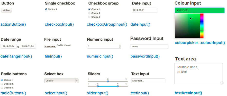
Adding Inputs to the UI
Now that we have data, we need to give our user the tools to explore
it. Shiny provides a wide variety of functions to create
Inputs. These functions all follow a similar naming
convention and structure. The function name will use camelCase with the
first part describing the input, and the second being the word “Input” -
such as selectInput(), sliderInput(), and
more.
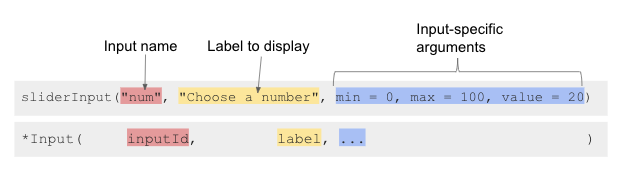
The function then takes an inputID argument - a string
which will be used to refer to the input later on in the server. Then a
label argument, for what the user will see as the text
describing the input. Finally, a wide variety of input specific
arguments. For example, see the following from Dean
Attali’s tutorial.
 For the purposes of our app,
let’s begin by adding a
For the purposes of our app,
let’s begin by adding a selectInput() to allow a user to
choose a year.
Callout
It would have been nice to have a slider for year. But, base Shiny
doesn’t have a function for that. You’d need
sliderTextInput() from shinyWidgets.
Looking at ?selectInput we see we will need the
following arguments:
-
inputId- a name for our input -
label- what the user sees -
choices- some choices for years. This can just be theunique()years from our data. -
selected = NULL- an default first year. For the moment, we will set it to the first year in our data.
Let’s insert the following in our sidebarPanel(),
replacing the text that was there, and see what it produces.
R
selectInput(
  inputID = "year",
  label = "Choose a year:",
  choices = unique(seagrass_casco$year) |> sort(),
  selected = unique(seagrass_casco$year) |> min() #to get the earliest year
)
You will note that we are using the data to populate this form. This
is good practice so that you don’t enter a value into your select that
isn’t found in the data, which can cause havoc. We also used
sort() so that our selector was in order.
R
checkboxGroupInput(
  inputId = "cover",
  label = "Percent Cover Classes:",
  choices = unique(seagrass_casco$cover_pct) |> sort(),
  selected =  unique(seagrass_casco$cover_pct) |> sort()
)
This is just the start of *Input() possibilities. Shiny
itself hosts a number of inputs, and there are multiple packages that
host other possible inputs.
Adding Placeholders for Outputs
Before we get to the business of creating outputs, we need to have
Shiny tell us where in the UI the outputs will be placed. To do this,
much like the *Input() functions, we have a series of
*Output() functions that will generate HTML placeholders
for where different outputs should go.
| Function | Output Type |
|---|---|
| plotOutput() | plot, ggplot |
| tableOutput() | table or data frame |
| uiOutput() | Shiny UI element |
| textOutput() | text |
| htmlOutput() | HTML code |
| leaflet::leafletOutput() | leaflet map |
Like inputs, these functions have a first argument - in this case
outputId which is a character string, and will be used
elsewhere in the app. Other arguemtns to these functions vary by output,
but can be used to do things like specify output window size, scaling,
and more. For the moment, let’s add two plotOutput()
windows to our app. One for a map - called “map” and one for a
histogram, called “hist”. This will go in our mainPanel()
as follows:
R
   mainPanel(
     plotOutput("map"),
     plotOutput("hist"),
   )
Note, if we had wanted to make these side by side, we could have used
column() or even gone hard on HTML with tables.
Render your app to make sure it works, but you will see that these areas will currently appear blank.
Servers and the Output
It is now time to dig into our server. Recall the code for the server looks like this:
R
# 3. define a server
server <- function(input, output) {}
It’s just an empty creation of a function. What happens inside the
function is what interests us. Note that the function takes two
arguments - input and output. These are the
names of lists that are part of the Shiny environment.
The list input stores all of the inputs from the
*Input() functions in the UI. The list output
will contain all of the outputs generated by functions in the server to
then plug into the UI above. All of the IDs we have in our
ui will be used as parts of these lists. So,
input$year will contain the value of year chosen.
output$map will contain the plot of a map to be displayed
in the UI.
So how do we generate output? Throughout our server we need to
continually add pieces to the output list that match what
is in the UI. These pieces should be generated by a series of
render*() functions. We have functions like
renderPlot(), renderTable(), etc. Note how
they are in many ways the inverse of the *Output()
functions above. render comes first - which is useful as it
reminds you that you are working in the server. But then the type of
output being generated has a direct match with a *Output()
function above. It makes it easy to search back and forth and to find
matching functions and elements.
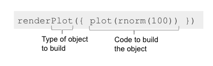 an
example render function from Dean Attali
an
example render function from Dean Attali
Note in the above function the argument to renderPlot()
is enclosed in {}. What? Curly braces? Why? Who? Don’t
worry. Think of them like fences to enclose a block of code. That block
of code is then passed to renderPlot() as a single
argument. The function knows how to handle and parse it. But, it only
wants one lump of code to work on. Formally, this argument is named
expr, but, that rarely gets used. As with all other
functions, render*() functions have other arguments that
can be supplied to fine-tune how they are executed.
Let’s modify our server to have sections for our outputs.
R
# 3. define a server
server <- function(input, output) {

  # our map block
  output$map <- renderPlot({

  })

  # our histogram block
  output$hist <- renderPlot({

  })


}
Now, in each block, we will need to filter our seagrass data down
based on input selection. This is going to require two
dplyr::filter() operations. The first to subset to year.
The second to subset to only those cover percent classes that are in the
cover percent selector. For both of these, we will reference our
input list - input$year and
input$cover. Let’s add that filter operation to both code
blocks.
R
# 3. define a server
server <- function(input, output) {

  # our map block
  output$map <- renderPlot({

    dat <- seagrass_casco |>
      filter(year == input$year) |>
      filter(cover_pct %in% input$cover)

  })

  # our histogram block
  output$hist <- renderPlot({

    dat <- seagrass_casco |>
      filter(year == input$year) |>
      filter(cover_pct %in% input$cover)
  })


}
Note, because these are two separate code blocks, we can reuse the
object name dat. In our next lesson, we will talk about how
to minimize copying and pasting code.
Finally, for each block, let’s add a ggplot(). In the
first, we will make a map based on geom_sf() with a good
polygon width and a viridis color scale. For the second, we will look at
the hectares of each bed.
R
# 3. define a server
server <- function(input, output) {

  # our map block
  output$map <- renderPlot({

    dat <- seagrass_casco |>
      filter(year == input$year) |>
      filter(cover_pct %in% input$cover)

    ggplot() +
      geom_sf(data = dat,
              linewidth = 1.5,
              color = "darkgreen")

  })

  # our histogram block
  output$hist <- renderPlot({

    dat <- seagrass_casco |>
      filter(year == input$year) |>
      filter(cover_pct %in% input$cover)

    ggplot(data = dat,
           aes(x = hectares)) +
      geom_histogram(bins = 50)
  })

}
Before you try and run this, remember to add
library(ggplot2) to your preamble.
ERROR
Error: package or namespace load failed for 'sf' in dyn.load(file, DLLpath = DLLpath, ...):
 unable to load shared object '/home/runner/.local/share/renv/cache/v5/R-4.3/x86_64-pc-linux-gnu/units/0.8-5/119d19da480e873f72241ff6962ffd83/units/libs/units.so':
  libudunits2.so.0: cannot open shared object file: No such file or directory
OUTPUT
Listening on http://127.0.0.1:3908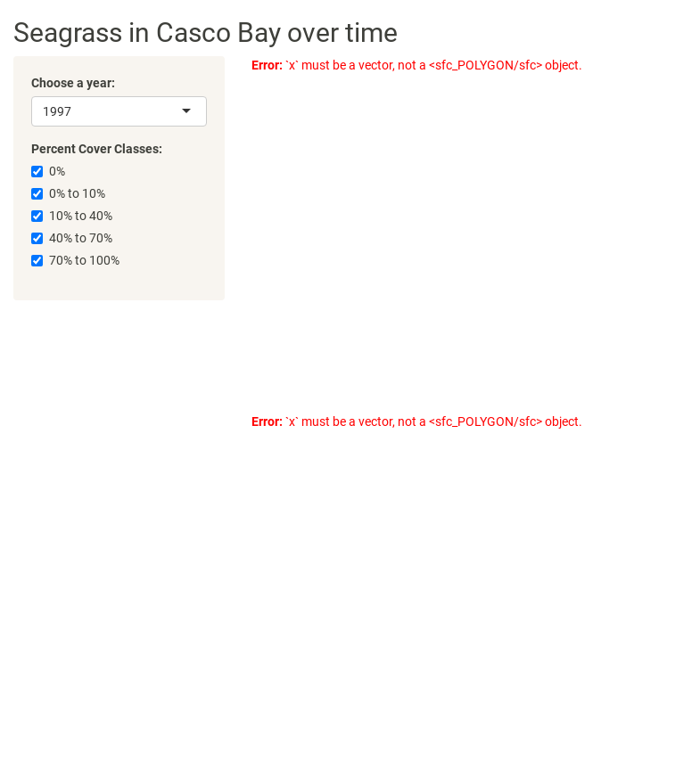
Oh No! Something Went Wrong with my Code!
As one last note, if you are running your code and it does not do
what you think it should do, the easiest way to begin the debugging
process is to see what objects you are working with in your
render*() calls. To do this, we can liberally sprinkle
print() statements in those calls. This will not return
text to the app, but rather will print to the console. So, if we put
print(input$year) in one of our render calls, whenever we
changed the year, it would print to the console. Later, when we upload
our app, we will see that it will print to the logfile for each run of
the app.
Key Points
- There are many types of inputs and outputs available for Shiny apps.
- Inputs follow a basic structure of having a
*Input()function with standard arguments in the UI. - Outputs have a placeholder in the UI using a
*Output()function. - Outputs are rendered in the server with a
render*()function. - The server has two lists to work with -
inputandoutput- which contain information for both.
Content from Reactive Objects in Shiny
Last updated on 2024-02-20 | Edit this page
Overview
Questions
- What is reactivity?
- How can I avoid re-processing data the same way for multiple outputs?
- How can I have inputs change in response to other inputs?
Objectives
- Explain what a reactive context means.
- Minimize code in our app with reactives.
Our App So Far
We have come far! Here is our app so far. It looks great, but, in reading it, notice that we re-use a whole block of code to filter data. Wouldn’t it be nice to instead only filter that data once, and not duplicate the effort?
R
# 1. Preamble
library(shiny)
library(shinythemes)
library(sf)
library(dplyr)
library(ggplot2)

seagrass_casco <- readRDS("data/joined_seagrass_cover.Rds")

# 2. Define a User Interface
ui <- fluidPage(
  title = "Seagrass in Casco App",
  theme = shinytheme("sandstone"),

 titlePanel("Seagrass in Casco Bay over time"),

 sidebarLayout(

   # sidebar
   sidebarPanel(
     selectInput(
       inputId = "year",
       label = "Choose a year:",
       choices = unique(seagrass_casco$year) |> sort(),
       selected = unique(seagrass_casco$year) |> min() #to get the earliest year
       ),

     checkboxGroupInput(
       inputId = "cover",
       label = "Percent Cover Classes:",
       choices = unique(seagrass_casco$cover_pct) |> sort(),
       selected =  unique(seagrass_casco$cover_pct) |> sort()
     ),
   ),

   # main
   mainPanel(
     plotOutput("map"),
     plotOutput("hist"),
   )
 )
)

# 3. define a server
server <- function(input, output) {

  # our map block
  output$map <- renderPlot({

    dat <- seagrass_casco |>
      filter(year %in% input$year) |>
      filter(cover_pct %in% input$cover)

    ggplot() +
      geom_sf(data = dat,
              linewidth = 1.5,
              color = "darkgreen")

  })

  # our histogram block
  output$hist <- renderPlot({

    dat <- seagrass_casco |>
      filter(year %in% input$year) |>
      filter(cover_pct %in% input$cover)

    ggplot(data = dat,
           aes(x = hectares)) +
      geom_histogram(bins = 50)
  })

}

shinyApp(ui = ui, server = server)
ERROR
Error: package or namespace load failed for 'sf' in dyn.load(file, DLLpath = DLLpath, ...):
 unable to load shared object '/home/runner/.local/share/renv/cache/v5/R-4.3/x86_64-pc-linux-gnu/units/0.8-5/119d19da480e873f72241ff6962ffd83/units/libs/units.so':
  libudunits2.so.0: cannot open shared object file: No such file or directory
Reactives
At its core, Shiny is all about reactivity
Reactivity is when you change the value of x, everything else that
relies on x is re-evaluated. In our app, output$map depends
on input$year. If you change input$year,
output$map changes. This is reactivity in action, and
input is a reactive variable.
This is not how things behave normally in R. For example
R
x <- 5
y <- x+10
x <- 10
y
OUTPUT
[1] 15Note that y is not 20. It is still 15.
Reactive Objects
In Shiny, we can make reactive objects that change in response to inputs inside of our server. For example, in the current app, if our server started like this
R
server <- function(input, output) {

 dat <- seagrass_casco |>
      filter(year %in% input$year) |>
      filter(cover_pct %in% input$cover)

...
And later on, in one of our render functions, we tried to use
dat, Shiny would throw an error. That’s because
dat as declared above is a static variable. It
does not change with context. Instead, we need to declare it a reactive
using reactive(), which works just like
render*(). We feed it a code block, and it generates a
reactive object.
R
server <- function(input, output) {

 dat <- reactive({
   seagrass_casco |>
      filter(year %in% input$year) |>
      filter(cover_pct %in% input$cover)
 })
...
We now have a reactive object. To use it, thought, we cannot call
dat as before. Instead, we use it like a function with no
arguments dat().
R
server <- function(input, output) {

 # reactives
 dat <- reactive({
   seagrass_casco |>
      filter(year %in% input$year) |>
      filter(cover_pct %in% input$cover)
 })
   # our map block
  output$map <- renderPlot({

    ggplot() +
      geom_sf(data = dat(),
              linewidth = 1.5,
              color = "darkgreen")

  })

  # our histogram block
  output$hist <- renderPlot({

    ggplot(data = dat(),
           aes(x = hectares)) +
      geom_histogram(bins = 50)
  })
}
Reactive UIs
Now that we can reactively filter our datasets, we can address a
second problem. Some years do not contain some cover_pct
classes. That means that it’s possible for us to select a value that
doesn’t exist. In our current app, this isn’t a complete killer, but, in
many other apps, dynamically generating inputs that match a range of
values in data can greatly simplify our UI.
This let’s us introduce a new render*() function,
renderUI(). This function allows us to create a UI element
based on inputs and reactives. We will need to make three changes to our
app code.
First, in our server, we need to modify our reactives. As this new UI element will depend on a data frame just filtered to year, we need to split our one reactive into two.
R
server <- function(input, output) {

 #reactives
 dat_year <- reactive({
   seagrass_casco |>
      filter(year %in% input$year)
 })

  dat <- reactive({
   dat_year |>
      filter(cover_pct %in% input$cover)
 })
...
Now filtering happens in two steps. The second reactive uses the
first. We can still use dat() as before in our other output
elements.
Second, we need to add a section to our server to create a UI object
with renderUI(). What’s nice is that we can take the old
code, paste it in here, and change seagrass_casco to
dat_year().
R
output$cover_checks <- renderUI({
  checkboxGroupInput(
    inputId = "cover",
    label = "Percent Cover Classes:",
    choices = unique(dat_year()$cover_pct) |> sort(),
    selected =  unique(dat_year()$cover_pct) |> sort()
  )

})
Last, we replace the checkboxGroupInput() in our
sidebarPanel() with
R
uiOutput("cover_checks")
Content from Making Shiny Apps Public
Last updated on 2024-02-20 | Edit this page
Overview
Questions
- How do I show the world my Shiny apps?
Objectives
- Publish your Shiny app
Shinyapps.io
In order to make your Shiny apps available to the world, we need to put them somewhere publicly accessible on the Worldwide Web. In order to do this, we need a Shiny Server - a server running R that knows how to deploy Shiny apps. While those of you with a server and know-how can deploy your own Shiny Server (it’s free!), that’s generally not an option for everyone.
For our purposes, we’re going to use Posit’s shinyapps.io, a free Shiny App hosting site that is integrated into R Studio.
Sign up for shinyapps.io
Go to shinyapps.io and take the steps to register for an account.
Other hosting options if you don’t run a server
There are other ways, but they require more technical expertise. If you are at or affiliated with a university, contact your scientific computing staff. They can setup a Shiny Server and Rstudio Server so you can easily deploy apps by uploading them.
If you don’t have that option, and shinyapps.io is not enough for you, you can deploy your app with Heroku or Digital Ocean. It’s going to take some work, patience, and desire to learn more about systems administration. Skills well worth learning.
Deploying Your App to Shinyapps.io
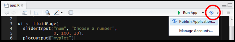 How to Publish your Shiny
App from Dean Attali
How to Publish your Shiny
App from Dean Attali
Deploying your app from within RStudio is fairly simple. Within
Rstudio, click the funky botton noted above (to the left of your code
pane) and select Publish Application. You will be walked
through steps to connect your instance of RStudio to shinyapps.io and then the app will
upload.
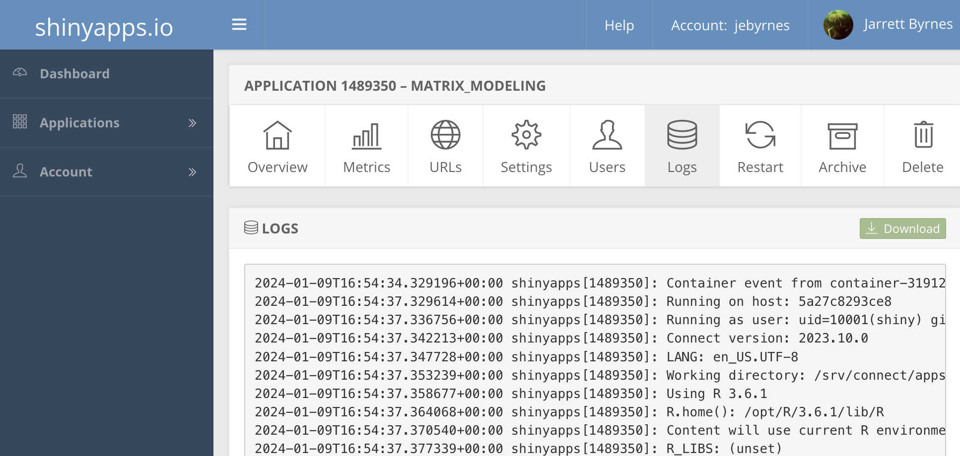
Run your app. If it has a problem, log into shinyapps.io and inspect the logfile for your app to see what went wrong.
Content from Translating a Shiny App
Last updated on 2024-02-20 | Edit this page
Overview
Questions
- How do I make my Shiny App accessible to non-English speakers?
Objectives
- Implement drop-down translations for Shiny
The Problem of Language
The entire world does not speak English.
While many developers might not be working in English, the default interface for Shiny contains many pieces that ARE in English. A wide variety of words that are programmed in, or are common terms of art that a developer might use are in English. Moreover, content written by a developer could well be in English.
While a user can use Google Translate - and might have to
for more complex grammer - giving them the power to even select
translation for the main words in your UI can be help broaden your
audience. Here we will explore two translation packages for Shiny. We
will start with a simple app which we can put in a file
app-translate.R.
library(shiny)
library(shi18ny)

ui <- fluidPage(
  h1("hello"),
  h3("to the world"),
  br(),
  tags$blockquote("more text")
  )

server <- function(input, output) {

}
Translating with shi18ny, Modules, and Reactives
shi18ny is an
older, but fairly solid, word-for-word translation engine. It has a large
dictionary of ~1,000 words in 18 languages. It’s not going to help
with complex grammer, but it’s idea for simple interfaces. Let’s start
by adding two pieces to the UI to get the language selector working. The
first is useShi18ny(). This just loads a lot of HTML code
that will be needed to do the translations. The second is a new input,
langSelectorInput(). We will use the
position = "Fixed" argument in order to have it not move
around as we scroll the page.
ui <- fluidPage(

  #language selector
  useShi18ny(),
  langSelectorInput("lang", position = "fixed", width = 200),


  h1("hello"),
  h3("to the world"),
  br(),
  tags$blockquote("more text")
)
That doesn’t seem to do anything, but that’s because translation is a bit different than other actions.
As the translation is dynamic, we can see that we want our translation to be reactive. Unlike reactives we have already looked at, something different is going on. First, we need to have a language translation system setup in the background. This seems like a block of code we could read in, but, we will need to place it in a specific context of a server or UI. This is a concept called a Shiny module.
So we will callModule(langSelector) with some additional
arguments for langSelector. One of which is
i18n - the list of languages. Let’s see how we implement
this with the server. See ?langSelector for more.
Last, we need a call to observeEvent() to make sure the
reactive change is seen. We have talked previously about reactives. We
can get the value from a reactive anytime in our code using the function
observe({}). This is very useful as within the code block,
we can insert some debug output - such as printing the value of a
reactive out. observeEvent({}) is similar, save that it
responds whenever a reactive experiences something “event-like”. It’s
useful for things like reactive buttons (to re-run a simulation), or
changing reactive dropdowns.
In this case, whenever the language chosen is changed, the languages
have to update across the entire page. Including the UI. So, we need to
run uiLangUpdate() with arguments to the classes the
library makes available and a call to the module itself.
server <- function(input, output) {
    # the language list
    i18n <- list(
      defaultLang = "en",
      availableLangs = c("es", "en", "pt")
    )

    # Call language module and save it as a reactive
    lang <- callModule(langSelector, "lang", i18n = i18n, showSelector = TRUE)

    observeEvent(lang(),{
      uiLangUpdate(input$shi18ny_ui_classes, lang())
    })
}
Now, changing the language selector didn’t actually change any of the
words. This is because Shiny needs to know WHICH words should be
translated. For this, we use the function ui_(). The
function takes a single string or vector of strings and, as long as each
have a match in the translation table, it will translate them as
needed.
ui <- fluidPage(

  #language selector
  useShi18ny(),
  langSelectorInput("lang", position = "fixed", width = 200),


  h1(ui_("hello")),
  h3(ui_("to"), ui_("the"), ui_("world") ),
  br(),
  tags$blockquote(ui_("more"), ui_("text"))
)
The continued repetition of the ui_() function gets a
bit annoying here. There are two solutions. Either provide the phrase
you want translated in an additional translation YAML file in a
directory or an additional CSV file in a directory called “locale”. Or,
we can make a uiOutput() and have the server do some
parsing of language with the i_() function.
So, we can change our UI to
ui <- fluidPage(

  #language selector
  useShi18ny(),
  langSelectorInput("lang", position = "fixed", width = 200),
  h1(ui_("hello")),

  uiOutput("more_text")

)
And our server to
server <- function(input, output) {
    # the language list
    i18n <- list(
      defaultLang = "en",
      availableLangs = c("es", "en", "pt")
    )

    # Call language module and save it as a reactive
    lang <- callModule(langSelector, "lang", i18n = i18n, showSelector = TRUE)

    observeEvent(lang(),{
      uiLangUpdate(input$shi18ny_ui_classes, lang())
    })

    output$more_text <- renderUI({
      list(
      h3(i_(c("to", "the", "world"), lang = lang())|> paste0(collapse = " ")),
      br(),
      tags$blockquote(i_(c("more", "text"), lang =lang())|> paste0(collapse = " "))
      )
    })

}
Translating Phrases with shiny.i18n
Going word by word can be tedious. What about whole phrases? What if
you have huge blocks of text and want to translate them - say, a whole
description. Enter the shiny.i18n
library. This library makes it simple for you to provide custom
translations for phrases and then tag them. You can supply these as
either a CSV or a JSON
file - a bunch of nested {} lists.
For example, here’s a CSV
en,it
Hello Shiny!,Ciao Shiny!
Tell me about seagrass!, Parlami delle erba marina!
This is fairly straightforward, and you can do it easily in excel, etc. BUT - for big, multi-line text blocks, it might become a bit of a pain in terms of line overruns, etc.
JSON
{
  "languages": ["en", "it"],
  "translation": [
      {
        "en": "Hello Shiny!",
        "it": "Ciao Shiny!"},
      {
        "en": "Tell me about seagrass!",
        "it": "Parlami delle erba marina!"
      }
    ]
}
Let’s download this json file into our toplevel directory.
shiny.i18n is a bit simpler to use than
shiny18ny, but similar in the how it integrates into an
app. First, we need to greate a Translator object in our
preamble. Do do this, we use Translator$new() to initialize
a new Translator object. We then use this new object to set the language
for the environment. Note, our Translator is something called an R6 object, which you don’t
need to worry about, save that it contains functions within itself.
Welcome to a soft introduction to Object
Oriented Programming.
R
# 1. Preamble
library(shiny)
library(shiny.i18n)

# Initialize the translator
trans_lang <- Translator$new(translation_json_path = "seagrass_it.json")

trans_lang$set_translation_language("en")
Now that we have a translator setup in our preamble,
trans_lan, we can use it in our UI. First, we need to use
the function usei18n(trans_lang) - our translator object -
to import a bunch of code that will handle the translation. Then, in our
UI, any phrase that can be translated can be wrapped into
trans_lang$t() which R will be able to translate later.
Finally, we need to put a selector for the language. To get the choices
for the languages available we can use
trans_lang$get_languages().
R
# 2. User interface
ui <- fluidPage(
  #import javascript
  usei18n(trans_lang),

  # the UI
  p(trans_lang$t("Hello Shiny!")),
  p(trans_lang$t("Tell me about seagrass!")),

  # A selector
  selectInput(
    "choose_language",
    "Select a language",
    choices = trans_lang$get_languages(),
    selected = "en"
  )

)
So, how do we make languages change? This is another case where we
need to use observeEvent() to observe a change in a
reactive and trigger a shange across the app. The function to change
languages is update_lang() which takes the argument of the
new language - here from input$choose_language.
R
# 3. Server
server <- function(input, output) {
  observeEvent(input$choose_language,{
    update_lang(input$choose_language)
  })
}
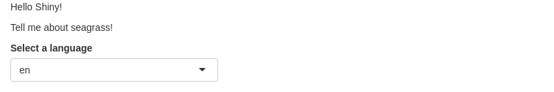
Putting these pieces together, we now have an app that can run and switch languages for large phrases.
Content from Spatial Selection
Last updated on 2024-02-20 | Edit this page
Overview
Questions
- How can I use interactive maps as an input select?
- How can I make my spatial apps more interactive?
Objectives
- Use leaflet in Shiny.
- Demonstrate the basic building blocks of a Shiny app.
Our App So Far
We’ve been doing great work on our app to look at seagrass beds in Casco Bay. Let’s summarize where we are so far, although we will remove the histogram for the moment.
R
# 1. Preamble
library(shiny)
library(shinythemes)
library(sf)
library(dplyr)
library(ggplot2)

seagrass_casco <- readRDS("data/joined_seagrass_cover.Rds")

# 2. Define a User Interface
ui <- fluidPage(
  title = "Seagrass in Casco App",
  theme = shinytheme("sandstone"),

 titlePanel("Seagrass in Casco Bay over time"),

 sidebarLayout(

   # sidebar
   sidebarPanel(
     selectInput(
       inputId = "year",
       label = "Choose a year:",
       choices = unique(seagrass_casco$year) |> sort(),
       selected = unique(seagrass_casco$year) |> min() #to get the earliest year
       ),

     checkboxGroupInput(
       inputId = "cover",
       label = "Percent Cover Classes:",
       choices = unique(seagrass_casco$cover_pct) |> sort(),
       selected =  unique(seagrass_casco$cover_pct) |> sort()
     ),
   ),

   # main
   mainPanel(
     plotOutput("map"),
   )
 )
)

# 3. define a server
server <- function(input, output) {

  # our map block
  output$map <- renderPlot({

    dat <- seagrass_casco |>
      filter(year %in% input$year) |>
      filter(cover_pct %in% input$cover)

    ggplot() +
      geom_sf(data = dat,
              linewidth = 1.5,
              color = "darkgreen")

  })


}
This is great, BUT, it could be improved greatly in two ways. First, why not have our map me more interactive - a leaflet map! Second, let’s actually add some color to our beds by cover.
Leaflet in Shiny Apps
Forunately, leaflet provides functions to work inside of
a Shiny app just like a plot. There is a leafletOutput()
and renderLeaflet() function. We can simply change the
plotOutput("map") in our UI to
leafletOutput("map"). Then, we can modify the server.
R
# 3. define a server
server <- function(input, output) {

  # our map block
  output$map <- renderLeaflet({

    dat <- seagrass_casco |>
      filter(year %in% input$year) |>
      filter(cover_pct %in% input$cover)

    leaflet() |>
      addProviderTiles("Esri.WorldTopoMap") |>
      addPolygons(data = dat,
                  color = "darkgreen",
                  weight = 1.5)

  })


}
Making a Reactive Leaflet Map
While this is awesome, as we can change our map easily, one frustration you might have noticed is that every time you change an input, the map resets its field of view. That’s because every time you change an input, Shiny re-runs the output, and it remakes the map from scratch. Not ideal.
Instead, we can use leafletProxy() to update a map. To
use leafletProxy(), we first create a map output with only
the parts of the map that will not respond to inputs. We can then treat
our map as a reactive object insofar as we will use
observe() to make changes are made. In our case, as our
selectors change the data used for the map, we will make the data a
reactive, and then use the reactive data for the observe()
statement.
Within our observe(), we will use
leafletProxy() with the argument mapId to
refer to the leaflet output - in this case "map". To it, we
will also have to add clearShapes() in order to plot only
what we are selecting. Otherwise, layers will be added on layers will be
added on layers will be….
Let’s look at our new server with the reactive, a static map (that includes bounds, as otherwise we’d start at a global scale), and our observe statement.
R
server <- function(input, output) {

  ## A reactive for data
  dat <- reactive({
    seagrass_casco |>
      filter(year %in% input$year) |>
      filter(cover_pct %in% input$cover)
  })

  ## An initial map with **only** elements that one' change
  output$map <- renderLeaflet({
    #we will need some initial bounds
    b <- st_bbox(seagrass_casco) |> as.numeric()

    leaflet() |>
      addProviderTiles("Esri.WorldTopoMap") |>
      fitBounds(b[1], b[2], b[3], b[4])

  })

  ## An observe statement to update the map
  observe({
    # here we use leafletProxy()
    leafletProxy(mapId = "map", data = dat()) |>
      clearShapes() |>
      addPolygons(
                  color = "darkgreen",
                  weight = 1.5)


  })

}
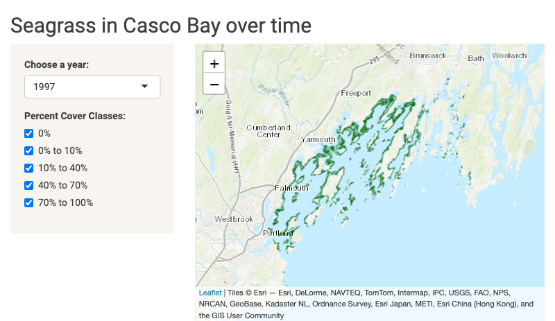
This now works as advertised!
Using Elements of a Leaflet Map as Input
As we have constructed a beautiful visualization of seagrass beds in Casco Bay, maybe we want to know more about each of those individual beds. We know that each polygon has a lot of information associated with it. For example.
R
seagrass_casco[1,]
Let’s say, for each bed, we want to be able to click on it and see
the information in that row of data. With leaflet maps, we can actually
do this without Shiny to some degree with the popup
argument. So, for example, we can make a map of 1997 with popups. We
will use paste() to make the text understandable.
R
seagrass_casco |>
  filter(year == 1997) |>
  leaflet() |>
  addTiles() |>
  addPolygons(popup = ~paste("Acres: ", acres))
We can do this for more than just acres. We can also use the
label argument to make this information popup when we just
mouse over the polygon.
This might be all you need! But, what if we want to do
something with the selected polygon data. Let’s say, for example,
we wanted to output the row of data the polygon came from. To do that,
we need to give each polygon an individual ID. Let’s add
bed_id column to the data that is just the row number. We
can put this in our preamble.
R
seagrass_casco <- seagrass_casco |>
  mutate(bed_id = 1:n())
To add this to our app, we can now add a layerId
argument to our polygon. We will use ~ to say that we are
going to evaluate one of the variables from
R
  ## An observe statement to update the map
  observe({
    # here we use leafletProxy()
    leafletProxy(mapId = "map", data = dat()) |>
      clearShapes() |>
      addPolygons(
                  color = "darkgreen",
                  weight = 1.5,
                  layerId = ~bed_id)


  })
So, now that we have layer IDs, how can we make them respond to
clicking on polygons? The answer is that interacting with
leaflet maps does trigger an input. We interact with maps
in two ways. One is with the whole map. The other is with just pieces.
Let’s focus on the later. The input triggered is
input$MAPID_OBJCATEGORY_EVENTNAMEwhere MAPID is the input ID of the map (here map),
OBJCATEGORY is a category descriptor of an object in a leaflet map. See
here for a
list of valid ones - what concerns us is shape and
marker. And last, EVENTNAME which is either
click, mouseover or mouseout.
So, for a click on a polygon, we’d be looking at
input$map_shape_clickTo show what this outputs, let’s insert two pieces into our code.
First, in the UI, add verbatimTextOutput("layer_click") and
to the server add
R
  output$layer_click <- renderText({
    capture.output(print(input$map_shape_click))
  })
From this, when we run the ap and click on a bed, we get output like this
$id [1] 3824 $.nonce [1] 0.8434182 $lat [1] 43.79836 $lng [1] -70.10101 OH! A list! With an ID which is the bed_id. We can do
something with that!
For the moment, let’s just show the hectares of the bed clicked on. We can do that by filtering to the bed ID and outputting text.
R
  output$layer_click <- renderText({
    one_row <- seagrass_casco |> filter(bed_id == input$map_shape_click$id)

    paste("This bed is", one_row$hectares, "hectares")
  })
Ew. What’s that initial output? To fix output when there is no click,
we need to return something for the NULL case.
R
  output$layer_click <- renderText({
    if(is.null(input$map_shape_click)) return("")

    one_row <- seagrass_casco |> filter(bed_id == input$map_shape_click)

    paste("This bed is", one_row$hectares, "hectares")
  })
Selecting With Your Map in Leaflet
What if, instead of what we’ve clicked on, we want information about
the area we are looking within? We have two options. The first is to use
the map itself as our selector. Like the
input$MAPID_OBJCATEGORY_EVENTNAME above, there is also just
an input$MAPID_EVENTNAME for the whole map.
These events include click which will return the
lat and lng of where you click,
center which does the same for where your map is centered,
zoom which will return your zoom level, and
bounds which will return the corner coordinates of your
map. north, east, south, and
west.
Below our text output in the UI, let’s add a
plotOutput("hectare_hist") and in our UI add a function
that crops our reactive dat() to the bounds of our
input$bounds. We can st_crop() with an
st_bbox() made from the bounds.
R
  # show the bed hectares
  output$hectare_hist <- renderPlot({
    # our crop box
    #xmin ymin xmax ymax
    crop_box <- st_bbox(c(xmin = input$map_bounds$west,
                        ymin = input$map_bounds$south,
                        xmax = input$map_bounds$east,
                        ymax = input$map_bounds$north),
                        crs = 4326)

    hist_data <- st_crop(dat(), crop_box)

    ggplot(data = hist_data, aes(x = hectares)) +
      geom_histogram(bins = 30)
  })
Selecting with a Draw Box
If you want to get fancy and use a drawing box instead, we need to
use something extra - the leaflet.extras
package. Lots of people have written Javascript extensions to Leaflet.
This package and leaflet.extras2
have tried to capture some of these into R. For our purposes, we need to
add an addDrawToolbar() to our map in the server.
R
  ## An initial map with **only** elements that one' change
  output$map <- renderLeaflet({
    #we will need some initial bounds
    b <- st_bbox(seagrass_casco) |> as.numeric()

    leaflet() |>
      addProviderTiles("Esri.WorldTopoMap") |>
      fitBounds(b[1], b[2], b[3], b[4]) |>
      addDrawToolbar(position = "topright",
                     editOptions =
                       editToolbarOptions(edit = FALSE))

  })
Note the editOptions. That’s just so we can have a trash
can to get rid of selectors once we are done.
This toolbar now produces the ability to draw shapes on a map and return information from them. Again, as above, using one of these will generate an input.
input$MAPID_draw_EVENTNAMEThere are a wide variety of EVENTNAME possibilities which are listed
here.
For our purposes, as we want to make a new histogram every time a square
is drawn, we want input$map_draw_new_feature which triggers
anytime a new feature is drawn.
What does this input return? Unfortunately, what it returns is a list
in the geojson format. Fortunately, we can use the geojsonsf
package to turn it into an sf object, and then crop as before to make
the histogram. Let’s change our histogram in our server to
R
  # show the bed hectares
  output$hectare_hist <- renderPlot({
    # good behavior
    if(is.null(input$map_draw_new_feature)) return(NA)

    # our crop box
    selected_shape <- input$map_draw_new_feature

    crop_sf <-
      geojsonsf::geojson_sf(jsonify::to_json(selected_shape, unbox = T))

    hist_data <- st_crop(dat(), crop_sf)

    ggplot(data = hist_data, aes(x = hectares)) +
      geom_histogram(bins = 30)
  })
And now take it for a spin!
Callout
That was a lot! For your future reference, here is the final code for the app by the end of this lesson. It’s a mid-sized app, but, a really nice one that accomplishes some very fancy tasks! Well done!
If you want to see a working version of it, try this link.
R
# 1. Preamble
library(shiny)
library(shinythemes)
library(sf)
library(dplyr)
library(ggplot2)
library(leaflet)
library(leaflet.extras)

seagrass_casco <- readRDS("data/joined_seagrass_cover.Rds")

seagrass_casco <- seagrass_casco |>
  mutate(bed_id = 1:n())


# 2. Define a User Interface
ui <- fluidPage(
  title = "Seagrass in Casco App",
  theme = shinytheme("sandstone"),

  titlePanel("Seagrass in Casco Bay over time"),

  sidebarLayout(

    # sidebar
    sidebarPanel(
      selectInput(
        inputId = "year",
        label = "Choose a year:",
        choices = unique(seagrass_casco$year) |> sort(),
        selected = unique(seagrass_casco$year) |> min() #to get the earliest year
      ),

      checkboxGroupInput(
        inputId = "cover",
        label = "Percent Cover Classes:",
        choices = unique(seagrass_casco$cover_pct) |> sort(),
        selected =  unique(seagrass_casco$cover_pct) |> sort()
      ),
    ),

    # main
    mainPanel(
      leafletOutput("map"),
      verbatimTextOutput("layer_click"),
      plotOutput("hectare_hist")
    )
  )
)

# 3. define a server
server <- function(input, output) {

  ## A reactive for data
  dat <- reactive({
    seagrass_casco |>
      filter(year %in% input$year) |>
      filter(cover_pct %in% input$cover)
  })

  ## An initial map with **only** elements that one' change
  output$map <- renderLeaflet({
    #we will need some initial bounds
    b <- st_bbox(seagrass_casco) |> as.numeric()

    leaflet() |>
      addProviderTiles("Esri.WorldTopoMap") |>
      fitBounds(b[1], b[2], b[3], b[4]) |>
      addDrawToolbar(position = "topright",
                     editOptions =
                       editToolbarOptions(edit = FALSE))

  })

  ## An observe statement to update the map
  observe({
    # here we use leafletProxy()
    leafletProxy(mapId = "map", data = dat()) |>
      clearShapes() |>
      addPolygons(
        color = "darkgreen",
        weight = 1.5,
        layerId = ~bed_id)


  })

  output$layer_click <- renderText({
    if(is.null(input$map_shape_click)) return("")

    one_row <- seagrass_casco |> filter(bed_id == input$map_shape_click$id)

    paste("This bed is", one_row$hectares, "hectares")
  })

  # show the bed hectares
  output$hectare_hist <- renderPlot({
    # good behavior
    if(is.null(input$map_draw_new_feature)) return(NA)

    # our crop box
    selected_shape <- input$map_draw_new_feature

    crop_sf <-
      geojsonsf::geojson_sf(jsonify::to_json(selected_shape, unbox = T))

    hist_data <- st_crop(dat(), crop_sf)

    ggplot(data = hist_data, aes(x = hectares)) +
      geom_histogram(bins = 30)
  })

}