Work with Multi-Band Rasters
Last updated on 2024-03-12 | Edit this page
WARNING
Warning in
download.file("https://www.naturalearthdata.com/http//www.naturalearthdata.com/download/110m/physical/ne_110m_graticules_all.zip",
: cannot open URL
'https://www.naturalearthdata.com/http//www.naturalearthdata.com/download/110m/physical/ne_110m_graticules_all.zip':
HTTP status was '500 Internal Server Error'
ERROR
Error in download.file("https://www.naturalearthdata.com/http//www.naturalearthdata.com/download/110m/physical/ne_110m_graticules_all.zip", : cannot open URL 'https://www.naturalearthdata.com/http//www.naturalearthdata.com/download/110m/physical/ne_110m_graticules_all.zip'Overview
Questions
- How can I visualize individual and multiple bands in a raster object?
Objectives
- Identify a single vs. a multi-band raster file.
- Import multi-band rasters into R using the
terrapackage. - Plot multi-band color image rasters in R using the
ggplotpackage.
First, some libraries you might not have loaded at the moment.
R
library(terra)
library(ggplot2)
library(dplyr)
library(tidyterra)
Things You’ll Need To Complete This Episode
See the lesson homepage for detailed information about the software, data, and other prerequisites you will need to work through the examples in this episode.
We introduced multi-band raster data in an earlier lesson. This episode explores how to import and plot a multi-band raster in R.
Getting Started with Multi-Band Data in R
In this episode, the multi-band data that we are working with is imagery collected using the Landsat 8 Satellite satellite on row 12 path 30 of it’s traverse around the planet. Landsat is a series of multispectral satellites with a 30m pixel resolution. This means that each image has multiple wavelengths of light observed - not just Red, Green, and Blue (RGB). Here are the bands of the Landsat 8 OLI:
- Band 1 Coastal Aerosol (0.43 - 0.45 µm) 30 m
- Band 2 Blue (0.450 - 0.51 µm) 30 m
- Band 3 Green (0.53 - 0.59 µm) 30 m
- Band 4 Red (0.64 - 0.67 µm) 30 m
- Band 5 Near-Infrared (0.85 - 0.88 µm) 30 m
- Band 6 SWIR 1(1.57 - 1.65 µm) 30 m
- Band 7 SWIR 2 (2.11 - 2.29 µm) 30 m
- Band 8 Panchromatic (PAN) (0.50 - 0.68 µm) 15 m
- Band 9 Cirrus (1.36 - 1.38 µm) 30 m
So, 4, 3, and 2 are RGB. By using the rast() function we
can read one raster bands (i.e. the first one) or many.
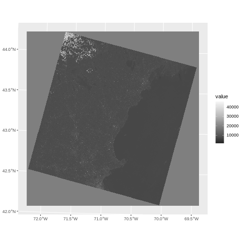
Let’s start by looking at the red band.
R
landsat_band4_1230 <-
  rast("data/landsat_casco/LC08_L2SP_012030_20230903_20230912_02_T1/LC08_L2SP_012030_20230903_20230912_02_T1_SR_B4.TIF")

ggplot() +
  geom_spatraster(data = landsat_band4_1230) +
  scale_fill_distiller(palette = "Greys")
R
landsat_band4_1230
OUTPUT
class       : SpatRaster
dimensions  : 7991, 7891, 1  (nrow, ncol, nlyr)
resolution  : 30, 30  (x, y)
extent      : 232485, 469215, 4662585, 4902315  (xmin, xmax, ymin, ymax)
coord. ref. : WGS 84 / UTM zone 19N (EPSG:32619)
source      : LC08_L2SP_012030_20230903_20230912_02_T1_SR_B4.TIF
name        : LC08_L2SP_012030_20230903_20230912_02_T1_SR_B4
Notice that when we look at the attributes of this band, we see:
dimensions : 7991, 7891, 1 (nrow, ncol, nlyr)
This is R telling us that we read only one band.
Raster Stacks in R
Next, we will work with mutiple bands as an R raster object. We will then plot a 3-band composite, or full color, image, and what is called a ‘fasle-color’ image.
To bring in all bands of a multi-band raster, we use
therast() function.
For multi-layer views, we need to look at all of the files we get with a typical sensor image. They are often listed as different files (although they can come in one big file.) Let’s see what a typical Landsat image has.
R
list.files("data/landsat_casco/LC08_L2SP_012030_20230903_20230912_02_T1/")
OUTPUT
 [1] "LC08_L2SP_012030_20230903_20230912_02_T1_ANG.txt"
 [2] "LC08_L2SP_012030_20230903_20230912_02_T1_MTL.txt"
 [3] "LC08_L2SP_012030_20230903_20230912_02_T1_MTL.xml"
 [4] "LC08_L2SP_012030_20230903_20230912_02_T1_QA_PIXEL.TIF"
 [5] "LC08_L2SP_012030_20230903_20230912_02_T1_QA_RADSAT.TIF"
 [6] "LC08_L2SP_012030_20230903_20230912_02_T1_SR_B1.TIF"
 [7] "LC08_L2SP_012030_20230903_20230912_02_T1_SR_B2.TIF"
 [8] "LC08_L2SP_012030_20230903_20230912_02_T1_SR_B3.TIF"
 [9] "LC08_L2SP_012030_20230903_20230912_02_T1_SR_B4.TIF"
[10] "LC08_L2SP_012030_20230903_20230912_02_T1_SR_B5.TIF"
[11] "LC08_L2SP_012030_20230903_20230912_02_T1_SR_B6.TIF"
[12] "LC08_L2SP_012030_20230903_20230912_02_T1_SR_B7.TIF"
[13] "LC08_L2SP_012030_20230903_20230912_02_T1_SR_QA_AEROSOL.TIF"
That’s a lot of files! To load them in with rast() in a
single object, thought, we will want only those that are TIF files, and
we will need the full path to each one. Fortunately,
list.files() makes that easy for us.
R
landsat_files <-
  list.files("data/landsat_casco/LC08_L2SP_012030_20230903_20230912_02_T1",
             full.names = TRUE,
             pattern = "TIF")

landsat_files
OUTPUT
 [1] "data/landsat_casco/LC08_L2SP_012030_20230903_20230912_02_T1/LC08_L2SP_012030_20230903_20230912_02_T1_QA_PIXEL.TIF"
 [2] "data/landsat_casco/LC08_L2SP_012030_20230903_20230912_02_T1/LC08_L2SP_012030_20230903_20230912_02_T1_QA_RADSAT.TIF"
 [3] "data/landsat_casco/LC08_L2SP_012030_20230903_20230912_02_T1/LC08_L2SP_012030_20230903_20230912_02_T1_SR_B1.TIF"
 [4] "data/landsat_casco/LC08_L2SP_012030_20230903_20230912_02_T1/LC08_L2SP_012030_20230903_20230912_02_T1_SR_B2.TIF"
 [5] "data/landsat_casco/LC08_L2SP_012030_20230903_20230912_02_T1/LC08_L2SP_012030_20230903_20230912_02_T1_SR_B3.TIF"
 [6] "data/landsat_casco/LC08_L2SP_012030_20230903_20230912_02_T1/LC08_L2SP_012030_20230903_20230912_02_T1_SR_B4.TIF"
 [7] "data/landsat_casco/LC08_L2SP_012030_20230903_20230912_02_T1/LC08_L2SP_012030_20230903_20230912_02_T1_SR_B5.TIF"
 [8] "data/landsat_casco/LC08_L2SP_012030_20230903_20230912_02_T1/LC08_L2SP_012030_20230903_20230912_02_T1_SR_B6.TIF"
 [9] "data/landsat_casco/LC08_L2SP_012030_20230903_20230912_02_T1/LC08_L2SP_012030_20230903_20230912_02_T1_SR_B7.TIF"
[10] "data/landsat_casco/LC08_L2SP_012030_20230903_20230912_02_T1/LC08_L2SP_012030_20230903_20230912_02_T1_SR_QA_AEROSOL.TIF"
Great! We can now load those in smoothly with
rast().
R
# load all bands
landsat_all_1230 <- rast(landsat_files)

landsat_all_1230
OUTPUT
class       : SpatRaster
dimensions  : 7991, 7891, 10  (nrow, ncol, nlyr)
resolution  : 30, 30  (x, y)
extent      : 232485, 469215, 4662585, 4902315  (xmin, xmax, ymin, ymax)
coord. ref. : WGS 84 / UTM zone 19N (EPSG:32619)
sources     : LC08_L2SP_012030_20230903_20230912_02_T1_QA_PIXEL.TIF
              LC08_L2SP_012030_20230903_20230912_02_T1_QA_RADSAT.TIF
              LC08_L2SP_012030_20230903_20230912_02_T1_SR_B1.TIF
              ... and 7 more source(s)
names       : LC08_~PIXEL, LC08_~ADSAT, LC08_~SR_B1, LC08_~SR_B2, LC08_~SR_B3, LC08_~SR_B4, ...
Now we have a very different set of dimensions and names.
dimensions : 7991, 7891, 10 (nrow, ncol, nlyr)
10 bands! To see what is loaded, we can just use
names()
R
names(landsat_all_1230)
OUTPUT
 [1] "LC08_L2SP_012030_20230903_20230912_02_T1_QA_PIXEL"
 [2] "LC08_L2SP_012030_20230903_20230912_02_T1_QA_RADSAT"
 [3] "LC08_L2SP_012030_20230903_20230912_02_T1_SR_B1"
 [4] "LC08_L2SP_012030_20230903_20230912_02_T1_SR_B2"
 [5] "LC08_L2SP_012030_20230903_20230912_02_T1_SR_B3"
 [6] "LC08_L2SP_012030_20230903_20230912_02_T1_SR_B4"
 [7] "LC08_L2SP_012030_20230903_20230912_02_T1_SR_B5"
 [8] "LC08_L2SP_012030_20230903_20230912_02_T1_SR_B6"
 [9] "LC08_L2SP_012030_20230903_20230912_02_T1_SR_B7"
[10] "LC08_L2SP_012030_20230903_20230912_02_T1_SR_QA_AEROSOL"We just want red, green, blue, and near-infrared for now - bands 2 through 5. Note how that corresponds to layers 4 through 7. So we can subset down.
R
landsat_colors_1230 <- subset(landsat_all_1230,
                              subset = 4:7)
Let’s preview the attributes of our stack object:
R
landsat_colors_1230
OUTPUT
class       : SpatRaster
dimensions  : 7991, 7891, 4  (nrow, ncol, nlyr)
resolution  : 30, 30  (x, y)
extent      : 232485, 469215, 4662585, 4902315  (xmin, xmax, ymin, ymax)
coord. ref. : WGS 84 / UTM zone 19N (EPSG:32619)
sources     : LC08_L2SP_012030_20230903_20230912_02_T1_SR_B2.TIF
              LC08_L2SP_012030_20230903_20230912_02_T1_SR_B3.TIF
              LC08_L2SP_012030_20230903_20230912_02_T1_SR_B4.TIF
              LC08_L2SP_012030_20230903_20230912_02_T1_SR_B5.TIF
names       : LC08_L2~1_SR_B2, LC08_L2~1_SR_B3, LC08_L2~1_SR_B4, LC08_L2~1_SR_B5
We can view the attributes of each band in the stack in a single output. For example, if we had hundreds of bands, we could specify which band we’d like to view attributes for using an index value:
R
landsat_colors_1230[[2]]
OUTPUT
class       : SpatRaster
dimensions  : 7991, 7891, 1  (nrow, ncol, nlyr)
resolution  : 30, 30  (x, y)
extent      : 232485, 469215, 4662585, 4902315  (xmin, xmax, ymin, ymax)
coord. ref. : WGS 84 / UTM zone 19N (EPSG:32619)
source      : LC08_L2SP_012030_20230903_20230912_02_T1_SR_B3.TIF
name        : LC08_L2SP_012030_20230903_20230912_02_T1_SR_B3
We can also use the ggplot functions to plota histogram
of the first (blue) band:
R
ggplot() +
  geom_histogram(data = landsat_colors_1230,
                 aes(x = LC08_L2SP_012030_20230903_20230912_02_T1_SR_B3),
                 bins = 1e4)
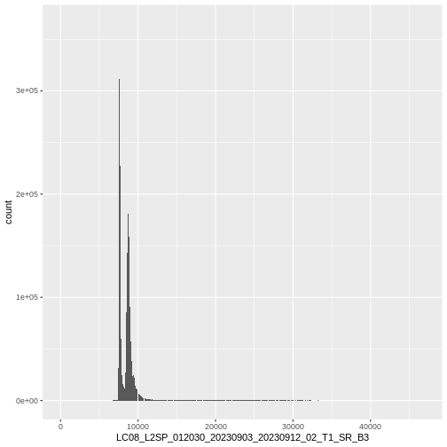
This tells us that, for example, we might want to cutoff high quantiles when we start to blend colors for an RGB plot.
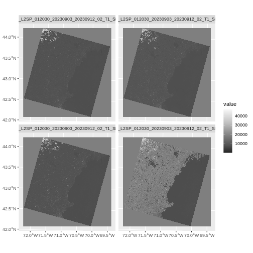
We can also plot all of the bands with either
plot() or ggplot() adding a
facet_wrap(facets = vars(lyr)) call to facet by layer.
R
#plot(landsat_colors_1230)

ggplot() +
  geom_spatraster(data = landsat_colors_1230) +
  facet_wrap(facets = vars(lyr)) +
  scale_fill_distiller(palette = "Greys")
R
ggplot() +
  geom_spatraster(data = landsat_colors_1230[[3:4]]) +
  facet_wrap(facets = vars(lyr)) +
  scale_fill_viridis_b()
We’d expect a brighter value for the land in band 5 (NIR) than in band 4 (red) because healthy vegetation reflects MORE NIR light than red light.
Create A Three Band Image
To render a final three band, colored image in R, we use the
plotRGB() or geom_spatraster_rgb()
function.
This function allows us to:
Identify what bands we want to render in the red, green and blue regions. The
plotRGB()function defaults to a 1=red, 2=green, and 3=blue band order. However, you can define what bands you’d like to plot manually. Manual definition of bands is useful if you have, for example a near-infrared band and want to create a color infrared image.Adjust the
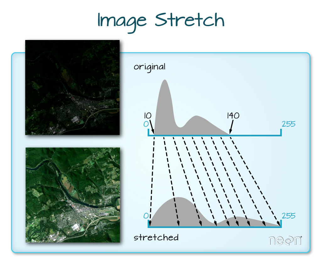
stretchof the image to increase or decrease contrast.
Let’s plot our 3-band image. Note that we can use the
plotRGB() function directly with our RasterStack object (we
don’t need a dataframe as this function isn’t part of the
ggplot2 package).
R
plotRGB(landsat_colors_1230,
        r = 3, g = 2, b = 1)
That throws an error as sometimes plotRGB doesn’t like really large values when it rescales. RGB values for a computer screen are typically between 0 and 255, so, we just need to rescale our values between 0 and 255. We can do that by multiplying the raster values by 255/(max of the raster values). Note, you can either do this so EACH channel is rescalled to 0-255, or, they are all rescaled by one grand value.
R
colmax <- max(landsat_colors_1230[[1:3]]) |> values() |> max(na.rm = TRUE)

colmax

plotRGB(landsat_colors_1230 * 255/colmax,
        r = 3, g = 2, b = 1, main = "Rescaled for each channel")
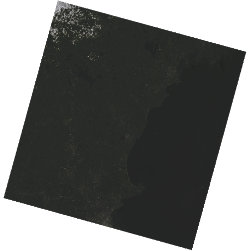
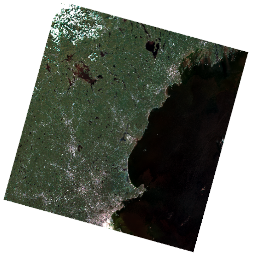
The image above looks OK, but dark. You can actually play with the
denominator of the scaling to make more interesting ones, or scale by
other rasters. But, there are more standard (and better) stretching
algorithms. We can explore whether applying a stretch to the image might
improve clarity and contrast using stretch="lin" or
stretch="hist".
When the range of pixel brightness values is closer to 0, a darker image is rendered by default. We can stretch the values to extend to the full 0-255 range of potential values to increase the visual contrast of the image.
When the range of pixel brightness values is closer to 255, a lighter image is rendered by default. We can stretch the values to extend to the full 0-255 range of potential values to increase the visual contrast of the image.
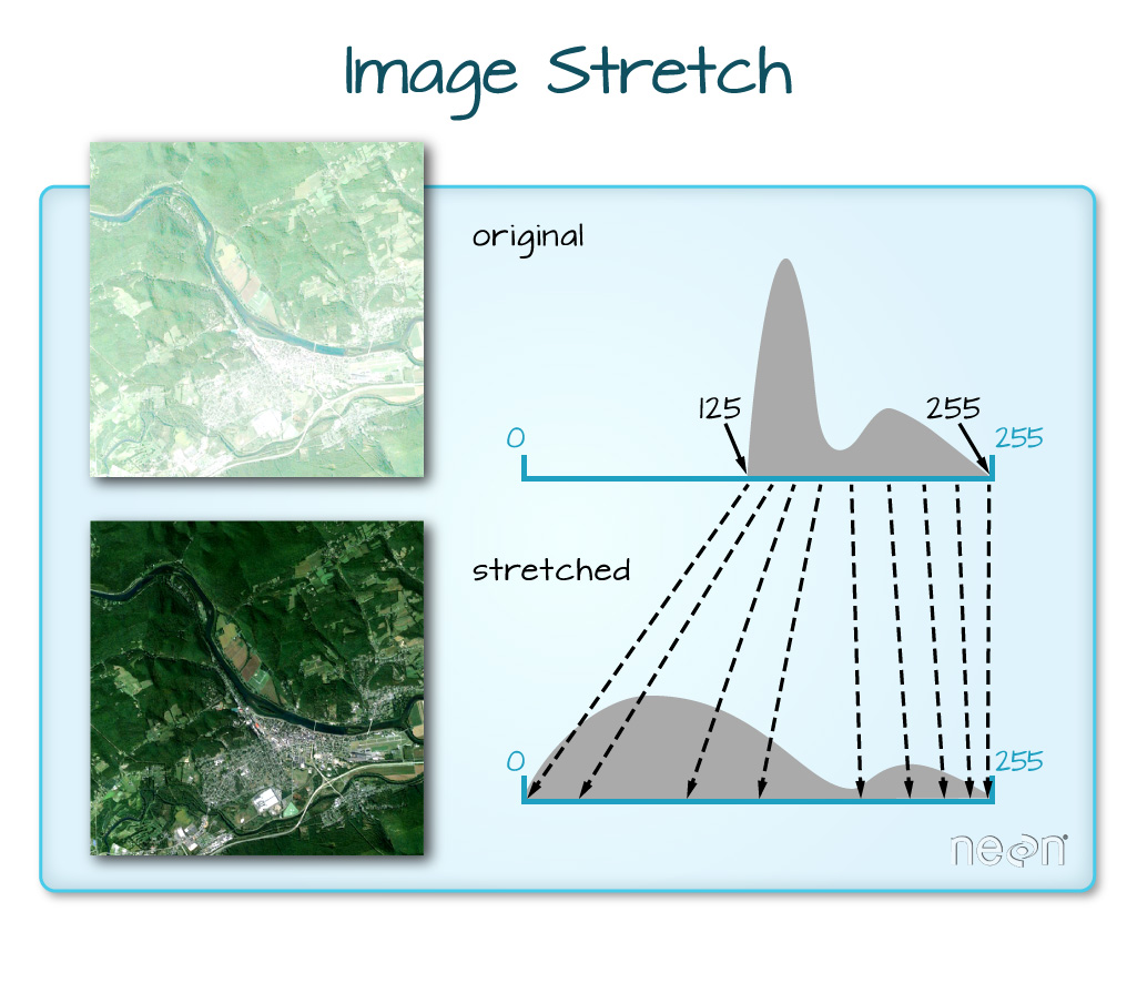
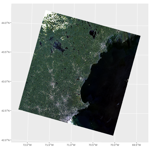
We can implement this easily in R where we not only make a linear stretch, but chop off some of the highest and lowest values.
R
plotRGB(landsat_colors_1230,
        r = 1, g = 2, b = 3,
        stretch = "lin")
If the problem is that we want an even distribution of values for
each channel, rather than clumps and clusters, we use hist
as our stretch.
R
plotRGB(landsat_colors_1230,
        r = 1, g = 2, b = 3,
        stretch = "hist")
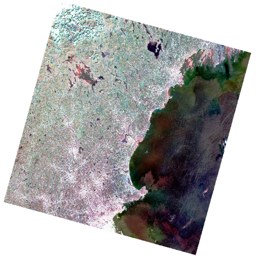
In this case, the stretch begins to show some things happening offshore a bit more, which might prompt more investigation.
Note, to do this with ggplot2, we need to apply
stretch() to the raster first and cut off the lower and
upper quantile of values. We can then use
geom_spatraster_rgb(). Note, to use stretch()
and get the RGB right, we need to reference the layer numbers of the
raster as indices.
R
ggplot() +
  geom_spatraster_rgb(data = stretch(landsat_colors_1230[[c(3,2,1)]],
                                 minq = 0.02, maxq = 0.98))
Challenge - False Color Images
What we have plotted above is a True Color Image. To help see things, many people use False color Images. Either they switch the bands (so, GRB instead of RGB) or use other bands. What do you see that is different if you try the following. Apply any stretch you like.
- Instead of RGB, plot GRB.
- Instead of RBG, plot NRG (where N = NIR). This creates a ‘vegetation in red’ map, which can be useful for vegetation.
- Note how we use r, g, and b as channel 1, 2, and 3.
R
plotRGB(landsat_colors_1230,
        r = 2, g = 3, b = 1,
        stretch = "lin")
- Here if you stretch with hist,you can get a better split between very vegetated and urbanized areas.
R
plotRGB(landsat_colors_1230,
        r = 4, g = 3, b = 2,
        stretch = "hist")
Data Tip
You can create interactive RGB overlays as well. But it takes some
extra doing, as you have to downsample large images, as
geom_spatraster() does natively. You can do this with
spatSample(). leaflet currently does odd
things to RGB rasters, so, you should use the leafem
library. Which does not yet handle SpatRaster objects from
terra. Fortunately, it’s a small thing to convert it to an
old school raster stack with raster::stack()
(we’re not loading the whole library to prevent conflicts in function
names). Note, for big rasters, you can up maxbytes in the
addRasterRGB from it’s default of 4*1024*1024,
but, this can cause plotting to take a very very very long time.
R
library(leaflet)
library(leafem)

# resample and then convert to a raster::stack object
# note, if this raster was small, we wouldn't have to
# spatSample()
landsat_colors_raster <- landsat_colors_1230 |>
  spatSample(size = 5e5, as.raster = TRUE, method = "regular")|>
  raster::stack()

# plot using addRasterRGB from leafem
leaflet() |>
  addRasterRGB(x = landsat_colors_raster,
               quantiles = c(0.02, 0.98))