Handling Spatial Projection & CRS
Last updated on 2024-03-12 | Edit this page
WARNING
Warning in
download.file("https://www.naturalearthdata.com/http//www.naturalearthdata.com/download/110m/physical/ne_110m_graticules_all.zip",
: cannot open URL
'https://www.naturalearthdata.com/http//www.naturalearthdata.com/download/110m/physical/ne_110m_graticules_all.zip':
HTTP status was '500 Internal Server Error'
ERROR
Error in download.file("https://www.naturalearthdata.com/http//www.naturalearthdata.com/download/110m/physical/ne_110m_graticules_all.zip", : cannot open URL 'https://www.naturalearthdata.com/http//www.naturalearthdata.com/download/110m/physical/ne_110m_graticules_all.zip'Overview
Questions
- How do I work with data sets that are in different projections?
Objectives
- Examine objects with different CRSs in the same plot.
- Reproject a raster and a vector layer in R.
- Plot vector and raster layers in the same plot.
Things You’ll Need To Complete This Episode
See the lesson homepage for detailed information about the software, data, and other prerequisites you will need to work through the examples in this episode.
Projection in R
In an earlier episodes we learned how to layer multiple vector data types. These principles extend to layering in raster data. When combining multiple data sources, particularly from different agencies or research efforts, we often find that they do not have the same Coordinate Reference System. This can be true of combining multiple vectors or rasters, or both.
We will apply our skills learned thus far to create maps that combine
both the coastline of Casco Bay (casco_coastline) with SST
data from 2022 (b10_casco_2022) and seagrass data
(seagrass_casco_2022). We will learn how to map vector data
sources that are in different CRSs and thus don’t line up on a map.
Load the Data
We will continue to use the sf and terra
packages in this episode as well as others from previously.
R
library(terra)
library(sf)
library(ggplot2)
library(tidyterra)
library(dplyr)
We will continue to work with the two ESRI shapefiles
that we loaded in the previously as well
as some Sea Surface Temperature data from our raster lessons.
R
# Casco Bay SST from Sept 9, 2022
b10_casco_2022 <- rast(
  "data/landsat_casco/b10_cropped/LC08_L2SP_011030_20220909_20220914_02_T1_ST_B10.TIF")

# Seagrass beds in 2022
seagrass_casco_2022 <- st_read(
  "data/maine_gov_seagrass/MaineDEP_Casco_Bay_Seagrass_2022/MaineDEP_Casco_Bay_Seagrass_2022.shp")

# Casco Coastline
casco_coastline <- st_read(
  "data/maine_gov_maps/Maine_State_Boundary_Polygon_Feature/Maine_State_Boundary_Polygon_Feature.shp") |>
  st_make_valid() |>
  st_crop(seagrass_casco_2022)
Working With Spatial Data From Different Sources
We often need to gather spatial datasets from different sources and/or data that cover different spatial extents. These data are often in different Coordinate Reference Systems (CRSs).
Some reasons for data being in different CRSs include:
- The data are stored in a particular CRS convention used by the data provider (for example, a government agency).
- The data are stored in a particular CRS that is customized to a region. For instance, many states in the US prefer to use a State Plane projection customized for that state.
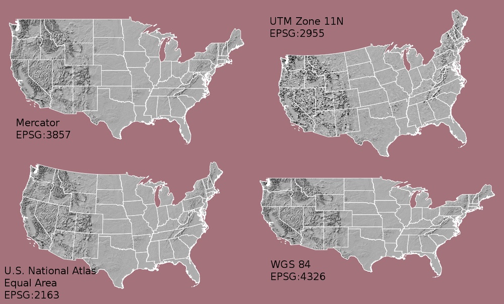
Notice the differences in shape associated with each different projection. These differences are a direct result of the calculations used to “flatten” the data onto a 2-dimensional map. Often data are stored purposefully in a particular projection that optimizes the relative shape and size of surrounding geographic boundaries (states, counties, countries, etc).
In this episode we will learn how to identify and manage spatial data in different projections. We will learn how to reproject the data so that they are in the same projection to support plotting / mapping. Note that these skills are also required for any geoprocessing / spatial analysis. Data need to be in the same CRS to ensure accurate results.
Inspecting CRS
To begin, how different are these two data sources? We can inspect their respective Coordinate Reference Systems to see.
R
crs(b10_casco_2022, proj = TRUE)
OUTPUT
[1] "+proj=utm +zone=19 +datum=WGS84 +units=m +no_defs"R
crs(casco_coastline, proj = TRUE)
OUTPUT
[1] "+proj=longlat +datum=WGS84 +no_defs"R
# st_crs(casco_coastline)$proj4string #this also works
Our project string for b10_casco_2022 specifies the UTM
projection as follows:
+proj=utm +zone=19 +datum=WGS84 +units=m +no_defs
- proj=utm: the projection is UTM, UTM has several zones.
- zone=19: the zone is 19
- datum=WGS84: the datum WGS84 (the datum refers to the 0,0 reference for the coordinate system used in the projection)
- units=m: the units for the coordinates are in METERS.
- no_defs: nothing is used from detault files.
Note that the zone is unique to the UTM projection. Not
all CRSs will have a zone.
For casco_coastline
Our project string for casco_coastline specifies the
lat/long projection as follows:
+proj=longlat +datum=WGS84 +no_defs
- proj=longlat: the data are in a geographic (latitude and longitude) coordinate system
- datum=WGS84: the datum WGS84 (the datum refers to the 0,0 reference for the coordinate system used in the projection)
- no_defs: nothing is used from detault files.
Note that there are no specified units above. This is because this geographic coordinate reference system is in latitude and longitude which is most often recorded in decimal degrees.
Sometimes you will also see ellps=WGS84: the ellipsoid (how the earth’s roundness is calculated) is WGS84.
The projections are very different. Refer to UTM versus UTM in the figure of the US above.
Do We Need to Reproject?
We can begin by trying to plot these datasets together. One of the
nice things about tidyterra and how ggplot2
works with sf objects is that it projects them to the same
CRS. So, if we try and plot these data sources together:
R
ggplot() +
  geom_spatraster(data = b10_casco_2022) +
  geom_sf(data = casco_coastline) +
  scale_fill_viridis_c()
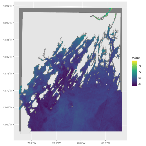
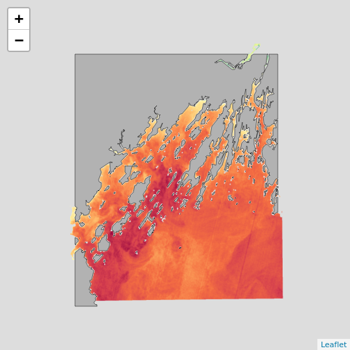
This looks pretty good. Leaflet looks good as well.
R
library(leaflet)

leaflet() |>
  addPolygons(data = casco_coastline,
              fill = "white", weight = 1,
              color = "black") |>
  addRasterImage(b10_casco_2022)
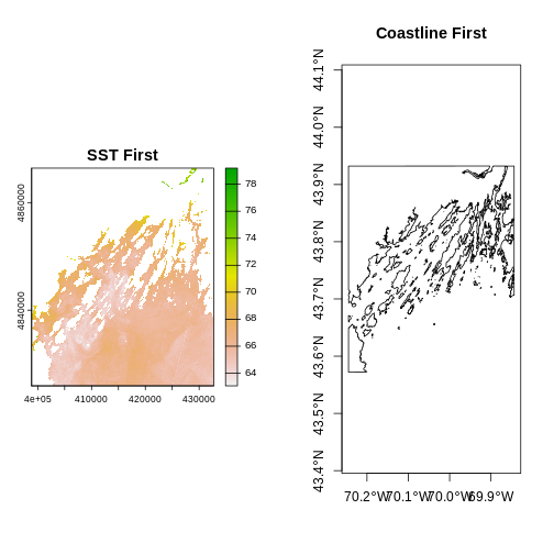
But, note two things. First, not every plotting algorithm will work.
For example if we went old school and used plot() with
add=TRUE to add a layer, this would have failed. Here we
see if putting a different layer down as the base.
R
par(mfrow = c(1,2))

plot(b10_casco_2022, main = "SST First")
plot(casco_coastline$geometry, add = TRUE)

plot(casco_coastline$geometry, main = "Coastline First", axes = TRUE)
plot(b10_casco_2022, add = TRUE)
R
par(mfrow = c(1,1))
Where did the other layer go? The axes give away that it’s a projection problem.
Second, in both of these, the borders and the raster don’t line up. So we want to line up extents. This is an aesthetic concern, but can be a big one - particularly if we were doing operations other than plotting. We need to crop one data set by the other.
Cropping and CRS
Cropping involves cutting off one part of an object to match another.
It is one of the operations we use to subset data spatially. We can also
extend objects to add rows or columns or mask out parts of an object. In
this case, let’s crop b10_casco_2022 so that we get rid of
that NA edge. After, we can crop the the coastline in order to eliminate
that weird hang-on piece of coast at the bottom of the maps.
As we are cropping a terra SpatRaster
object, we will use crop() which takes an input raster and
then an object with an extent to crop it to.
R
b10_casco_2022_cropped <- crop(b10_casco_2022,
                               casco_coastline)
ERROR
Error: [crop] extents do not overlapWell that’s odd. What are their extents?
R
ext(b10_casco_2022)
OUTPUT
SpatExtent : 398865, 432705, 4825935, 4866405 (xmin, xmax, ymin, ymax)R
ext(casco_coastline)
OUTPUT
SpatExtent : -70.244637867776, -69.843989726984, 43.5721328168498, 43.9322969014411 (xmin, xmax, ymin, ymax)Those are very different numbers due to their different CRS’s that we looked at above. This means, we will have to REPROJECT one of the two objects in order to crop it successfully, and then work in a common CRS.
Which data source should I reproject?
Projection works on a pixel by pixel basis. That means that for every pixel in your data, your computer will be doing work. As your data sets increase in size, projection can be computationally very expensive. In these cases, think about which layer will process faster. Often, it’s faster to project vector data, as it contains a tiny fraction of the points that are found in a raster data set.
While we can write a long CRS string, it’s easier to just take it
from an object or specify what’s called an EPSG code from epsg.org. We can see those codes
using crs() from terra with
describe = TRUE
R
crs(casco_coastline, describe = TRUE)
OUTPUT
    name authority code area         extent
1 WGS 84      EPSG 4326 <NA> NA, NA, NA, NA
From this we can see the EPSG code is 4326.
For the SST data…
R
crs(b10_casco_2022, describe = TRUE)
OUTPUT
                   name authority  code
1 WGS 84 / UTM zone 19N      EPSG 32619
                                                                                                                                                                                                                                                                                                                         area
1 Between 72°W and 66°W, northern hemisphere between equator and 84°N, onshore and offshore. Aruba. Bahamas. Brazil. Canada - New Brunswick (NB); Labrador; Nunavut; Nova Scotia (NS); Quebec. Colombia. Dominican Republic. Greenland. Netherlands Antilles. Puerto Rico. Turks and Caicos Islands. United States. Venezuela
           extent
1 -72, -66, 84, 0
the EPSG code is 32619.
Regardless, we can reproject the raster to the same projection as the coastline.
R
b10_casco_2022_4326 <- project(b10_casco_2022,
                               crs(casco_coastline))

b10_casco_2022_4326
OUTPUT
class       : SpatRaster
dimensions  : 1159, 1343, 1  (nrow, ncol, nlyr)
resolution  : 0.0003176554, 0.0003176554  (x, y)
extent      : -70.26025, -69.83364, 43.57953, 43.94769  (xmin, xmax, ymin, ymax)
coord. ref. : lon/lat WGS 84 (EPSG:4326)
source(s)   : memory
name        : SST_F_20220909
min value   :       63.06477
max value   :       79.34391
Note the difference in information about the projection (and EPSG code).
To transform sf vector data, we would have used the
function st_transform().
Proj4 & CRS Resources
- Official PROJ library documentation
- More information on the proj4 format.
- A fairly comprehensive list of CRSs by format.
- To view a list of datum conversion factors type:
sf_proj_info(type = "datum")into the R console. However, the results would depend on the underlying version of the PROJ library.
Cropping and Plotting
Now we can crop. We will first crop the SST raster to the coastline in order to get rid of the NA area in the raster.
R
b10_casco_2022_4326_cropped <- crop(b10_casco_2022_4326,
                                    casco_coastline)
Then we will crop the coastline to the cropped raster in order to get rid of that little bit of coast on the southern end.
R
casco_coastline_cropped <- st_crop(casco_coastline,
                                   b10_casco_2022_4326_cropped)
Let’s plot it and see if all of the effort was worth it!
R
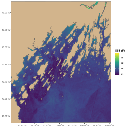
ggplot() +
  geom_spatraster(data = b10_casco_2022_4326_cropped) +
  geom_sf(data = casco_coastline_cropped, fill = "tan") +
  scale_fill_viridis_c() +
  labs(fill = "SST (F)") +
  coord_sf(expand = FALSE)
Summary: When CRS Attacks
The workflow outlined here, while in depth, is actually relatively simple. When you have two or more spatial data sets that you want to line up in terms of extent and projection.
- Determine if they actually differ in projection. If not, skip to 2.
- Reproject the smaller data source to the CRS of the larger one (if size is a concern).
- Crop back and forth to line up extents.
- Plot!
Challenge - Show us the temperature of seagrass beds
Let’s combine our SST and Seagrass data from 2022 to see if seagrasses are in warm places around Mackworth. Let’s start by making a Macworth Island AOI. We will do this by making a bounding box, and then turning it into an sf object.
R
mackworth_aoi <- st_bbox(c(xmin = -70.24768051612979,
                           xmax = -70.19432151530208,
                           ymin = 43.66353031177649,
                           ymax = 43.714022044471584),
                         crs = 4326) |>
  st_as_sfc()
Reproject the AOI and seagrass data to the same projection as the SST raster. Note, to get the CRS in a format
sfrecognizes, usest_crs(). We can leave out the coast.Crop everything to the Mackworth AOI. Note,
sfusesst_crop()whileterrausescrop.Plot! Try leaving seagrass polygons with an
NAfill to see the temperature inside and outside of the beds. As land is NA here, you can use thena.valueargument to yourscale_fill_*()to make the land tan.
- Reprojection
R
seagrass_casco_2022_32619 <- st_transform(seagrass_casco_2022,
                                          st_crs(b10_casco_2022))

mackworth_32619 <- st_transform(mackworth_aoi,
                              st_crs(b10_casco_2022))
- Cropping
R
seagrass_casco_2022_32619_mackworth <- st_crop(seagrass_casco_2022_32619,
                                               mackworth_32619)

b10_casco_2022_mackworth <- crop(b10_casco_2022,
                                 mackworth_32619)
- Plot!
R
ggplot() +
  geom_spatraster(data = b10_casco_2022_mackworth) +
  geom_sf(data = seagrass_casco_2022_32619_mackworth,
          color = "black",
          linewidth = 1,
          fill = NA) +
  scale_fill_viridis_c(na.value = "tan") +
  coord_sf(expand = FALSE)
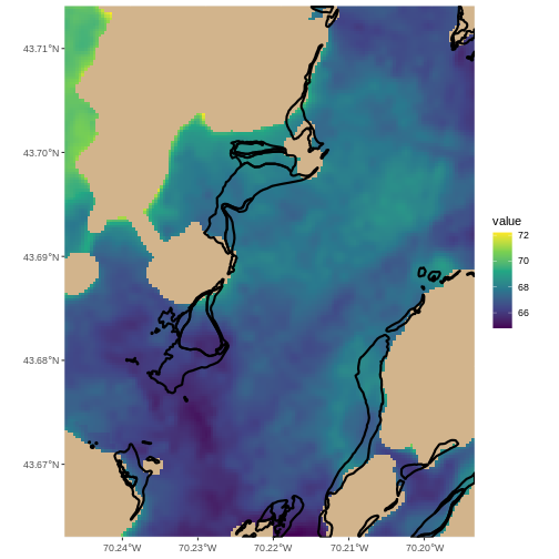
Looks like they are not in the warmest spots, but generally waters that in this Landsat scene were a bit cooler.
Key Points
- Multi-layered plots can combine vector and raster data sets.
-
ggplot2automatically converts all objects in a plot to the same CRS. - Still be aware of the CRS and extent for each object.
-
project()andst_transform()will reproject raster and vector data. -
crop()andst_crop()will crop raster and vector data.