Explore and Plot by Vector Layer Attributes
Last updated on 2024-03-12 | Edit this page
WARNING
Warning in
download.file("https://www.naturalearthdata.com/http//www.naturalearthdata.com/download/110m/physical/ne_110m_graticules_all.zip",
: cannot open URL
'https://www.naturalearthdata.com/http//www.naturalearthdata.com/download/110m/physical/ne_110m_graticules_all.zip':
HTTP status was '500 Internal Server Error'
ERROR
Error in download.file("https://www.naturalearthdata.com/http//www.naturalearthdata.com/download/110m/physical/ne_110m_graticules_all.zip", : cannot open URL 'https://www.naturalearthdata.com/http//www.naturalearthdata.com/download/110m/physical/ne_110m_graticules_all.zip'Overview
Questions
- How can I compute on the attributes of a spatial object?
Objectives
- Query attributes of a spatial object.
- Subset spatial objects using specific attribute values.
- Plot a vector feature, colored by unique attribute values.
Things You’ll Need To Complete This Episode
See the lesson homepage for detailed information about the software, data, and other prerequisites you will need to work through the examples in this episode.
This episode continues our discussion of vector layer attributes and covers how to work with vector layer attributes in R. It covers how to identify and query layer attributes, as well as how to subset features by specific attribute values. Finally, we will learn how to plot a feature according to a set of attribute values. We will do this looking at data regarding Seagrass beds in Casco Bay from 2022 provided by the Maine DEP. For full metadata, see here.
Load the Data
We will continue using the sf and ggplot2
packages in this episode. Make sure that you have these packages
loaded.
R
library(ggplot2)
library(dplyr)
library(sf)
We will continue to work with the ESRI shapefiles
(vector layers). Let’s start looking at seagrass beds around Casco Bay
from 2022.
R
# seagrass in 2022
seagrass_casco_2022 <- st_read(
  "data/maine_gov_seagrass/MaineDEP_Casco_Bay_Seagrass_2022/MaineDEP_Casco_Bay_Seagrass_2022.shp")
Query Vector Feature Metadata
As we discussed in the Open and Plot Vector Layers in R episode, we can view metadata associated with an R object using:
-
st_geometry_type()- The type of vector data stored in the object. -
nrow()- The number of features in the object -
st_bbox()- The spatial extent (geographic area covered by) of the object. -
st_crs()- The CRS (spatial projection) of the data.
We started to explore our seagrass_casco_2022 object To
see a summary of all of the metadata associated with our
seagrass_casco_2022 object, we can view the object with
View(seagrass_casco_2022) or print a summary of the object
itself to the console.
R
seagrass_casco_2022
OUTPUT
Simple feature collection with 622 features and 15 fields
Geometry type: POLYGON
Dimension:     XY
Bounding box:  xmin: -70.24464 ymin: 43.57213 xmax: -69.84399 ymax: 43.93221
Geodetic CRS:  WGS 84
First 10 features:
   OBJECTID Id Name       Acres   Hectares Orth_Cover Cover_Pct Field_Ver
1         1  1   01  0.04456005 0.01803281          1      0-10         Y
2         2  4   02  0.06076669 0.02459141          3     40-70         Y
3         3  6   03  2.56218247 1.03687846          3     40-70         Y
4         4  8   05  0.71816162 0.29062970          3     40-70         Y
5         5  9   06  0.01815022 0.00734513          3     40-70         Y
6         6 10   07  0.33051475 0.13375458          3     40-70         Y
7         7 11   08  0.08088664 0.03273366          1      0-10         Y
8         8 13   09  0.66689055 0.26988103          1      0-10         Y
9         9 14   10  0.03080650 0.01246695          3     40-70         Y
10       10 15   11 12.54074080 5.07505774          4    70-100         Y
   Video_YN                          Video Comment        Species
1         Y                            A03    <NA> Zostera marina
2         Y                            A04    <NA> Zostera marina
3         Y                            A05    <NA> Zostera marina
4         Y                            A07    <NA> Zostera marina
5         Y                            A08    <NA> Zostera marina
6         Y                            A09    <NA> Zostera marina
7         Y                            A10    <NA> Zostera marina
8         Y                            A11    <NA> Zostera marina
9         Y                            A12    <NA> Zostera marina
10        Y A14, A15, A16, A17, SP07, SP08    <NA> Zostera marina
                                 GlobalID  ShapeSTAre ShapeSTLen
1  {7CAB9D54-4BF9-4B91-94D6-4F0EA4AD53C1}   180.32842  102.57257
2  {D5396F39-D508-45CB-BFE0-13A506D4E94C}   245.91500   84.35420
3  {3C1ED4DC-6580-4CAC-9499-32D445019068} 10368.78375  719.04025
4  {6C1395B8-F532-46C6-AFBA-23B14C2F2E02}  2906.29561  315.88722
5  {EDEDAFA1-8605-4FAC-910F-E6E864F51209}    73.45108   34.00204
6  {820DE3B5-BA6E-4415-A110-95F9F94A4F1C}  1337.54527  165.98655
7  {E4E2A155-7B1C-46C3-94B5-6D0E58B1FEBB}   327.33664  112.52478
8  {C7FEF8AC-9BA7-429C-A45B-270E836FBBA1}  2698.81099  295.01388
9  {356C58A4-DB72-445F-83DA-1035C8EAE917}   124.66947   43.47523
10 {C797140E-F9CB-4EA0-9D7C-FBEA50FE9EB2} 50750.58217 1949.02908
                         geometry
1  POLYGON ((-70.20081 43.5722...
2  POLYGON ((-70.20228 43.5869...
3  POLYGON ((-70.20858 43.5909...
4  POLYGON ((-70.21488 43.5924...
5  POLYGON ((-70.21499 43.5931...
6  POLYGON ((-70.21582 43.5963...
7  POLYGON ((-70.21618 43.5964...
8  POLYGON ((-70.21641 43.5971...
9  POLYGON ((-70.21498 43.6063...
10 POLYGON ((-70.22445 43.6425...
We can use the ncol function to count the number of
attributes associated with a spatial object too. Note that the geometry
is just another column and counts towards the total.
R
ncol(seagrass_casco_2022)
OUTPUT
[1] 16We can view the individual name of each attribute using the
names() function in R:
R
names(seagrass_casco_2022)
OUTPUT
 [1] "OBJECTID"   "Id"         "Name"       "Acres"      "Hectares"
 [6] "Orth_Cover" "Cover_Pct"  "Field_Ver"  "Video_YN"   "Video"
[11] "Comment"    "Species"    "GlobalID"   "ShapeSTAre" "ShapeSTLen"
[16] "geometry"
We could also view just the first 6 rows of attribute values using
the head() function to get a preview of the data:
R
head(seagrass_casco_2022)
OUTPUT
Simple feature collection with 6 features and 15 fields
Geometry type: POLYGON
Dimension:     XY
Bounding box:  xmin: -70.21582 ymin: 43.57213 xmax: -70.20057 ymax: 43.59667
Geodetic CRS:  WGS 84
  OBJECTID Id Name      Acres   Hectares Orth_Cover Cover_Pct Field_Ver
1        1  1   01 0.04456005 0.01803281          1      0-10         Y
2        2  4   02 0.06076669 0.02459141          3     40-70         Y
3        3  6   03 2.56218247 1.03687846          3     40-70         Y
4        4  8   05 0.71816162 0.29062970          3     40-70         Y
5        5  9   06 0.01815022 0.00734513          3     40-70         Y
6        6 10   07 0.33051475 0.13375458          3     40-70         Y
  Video_YN Video Comment        Species                               GlobalID
1        Y   A03    <NA> Zostera marina {7CAB9D54-4BF9-4B91-94D6-4F0EA4AD53C1}
2        Y   A04    <NA> Zostera marina {D5396F39-D508-45CB-BFE0-13A506D4E94C}
3        Y   A05    <NA> Zostera marina {3C1ED4DC-6580-4CAC-9499-32D445019068}
4        Y   A07    <NA> Zostera marina {6C1395B8-F532-46C6-AFBA-23B14C2F2E02}
5        Y   A08    <NA> Zostera marina {EDEDAFA1-8605-4FAC-910F-E6E864F51209}
6        Y   A09    <NA> Zostera marina {820DE3B5-BA6E-4415-A110-95F9F94A4F1C}
   ShapeSTAre ShapeSTLen                       geometry
1   180.32842  102.57257 POLYGON ((-70.20081 43.5722...
2   245.91500   84.35420 POLYGON ((-70.20228 43.5869...
3 10368.78375  719.04025 POLYGON ((-70.20858 43.5909...
4  2906.29561  315.88722 POLYGON ((-70.21488 43.5924...
5    73.45108   34.00204 POLYGON ((-70.21499 43.5931...
6  1337.54527  165.98655 POLYGON ((-70.21582 43.5963...
To understand what these columns mean, we can refer back to the original metadata that gives a better description.
Challenge: Attributes for Different Spatial Classes
Explore the attributes associated with the roads_maine
and aoi_boundary_casco spatial objects.
How many attributes does each have?
What is the maximum speed posted speed limit on any road in Maine?
Which of the following is NOT an attribute of the
roads_mainedata object?
- Speed Limit B) County C) Road Length
- To find the number of attributes, we use the
ncol()function:
R
roads_maine <- st_read("data/maine_gov_maps/MaineDOT_Public_Roads/MaineDOT_Public_Roads.shp")
OUTPUT
Reading layer `MaineDOT_Public_Roads' from data source
  `/home/runner/work/r-raster-vector-geospatial/r-raster-vector-geospatial/site/built/data/maine_gov_maps/MaineDOT_Public_Roads/MaineDOT_Public_Roads.shp'
  using driver `ESRI Shapefile'
Simple feature collection with 100669 features and 30 fields
Geometry type: LINESTRING
Dimension:     XY
Bounding box:  xmin: -71.04662 ymin: 43.06728 xmax: -66.95202 ymax: 47.35999
Geodetic CRS:  WGS 84
R
ncol(roads_maine)
OUTPUT
[1] 31- Ownership information is in a column named
Ownership:
R
max(roads_maine$speed_lim, na.rm = TRUE)
OUTPUT
[1] 75- To see a list of all of the attributes, we can use the
names()function:
R
names(roads_maine)
OUTPUT
 [1] "OBJECTID"   "link_id"    "faadt"      "aadt_type"  "fed_urbrur"
 [6] "strtname"   "capacity"   "jurisdictn" "num_lanes"  "offic_mile"
[11] "st_urbrur"  "fedfunccls" "speed_lim"  "speedsrc"   "nhs_status"
[16] "priority"   "prirtecode" "prim_bmp"   "prim_emp"   "prirtename"
[21] "segment_id" "sh_sa_ir"   "townname"   "towncode"   "cntyname"
[26] "cnty_no"    "surfc_type" "dot_region" "dot_regi_1" "Shape_Leng"
[31] "geometry"
“Road Length” is not an attribute of this object.
Explore Values within One Attribute
We can explore individual values stored within a particular
attribute. Comparing attributes to a spreadsheet or a data frame, this
is similar to exploring values in a column. We did this with the
gapminder dataframe in an
earlier lesson. For spatial objects, we can use the same syntax:
objectName$attributeName.
First, what do we have to work with?
R
names(seagrass_casco_2022)
OUTPUT
 [1] "OBJECTID"   "Id"         "Name"       "Acres"      "Hectares"
 [6] "Orth_Cover" "Cover_Pct"  "Field_Ver"  "Video_YN"   "Video"
[11] "Comment"    "Species"    "GlobalID"   "ShapeSTAre" "ShapeSTLen"
[16] "geometry"
To see only unique values within the Cover_Pct field, we
can use the unique() function for extracting the possible
values of a character variable (R also is able to handle categorical
variables called factors; we worked with factors a little bit in an
earlier lesson.
R
unique(seagrass_casco_2022$Cover_Pct)
OUTPUT
[1] "0-10" "40-70" "70-100" "10-40" Subset Features
We can use the filter() function from dplyr
that we worked with in an earlier
lesson to select a subset of features from a spatial object in R,
just like with data frames.
For example, we might be interested only in features that are of
Hectares greater than 25. Once we subset out this data, we
can use it as input to other code so that code only operates on the
footpath lines.
R
large_beds <- seagrass_casco_2022 |>
  filter(Hectares > 25)

nrow(large_beds)
OUTPUT
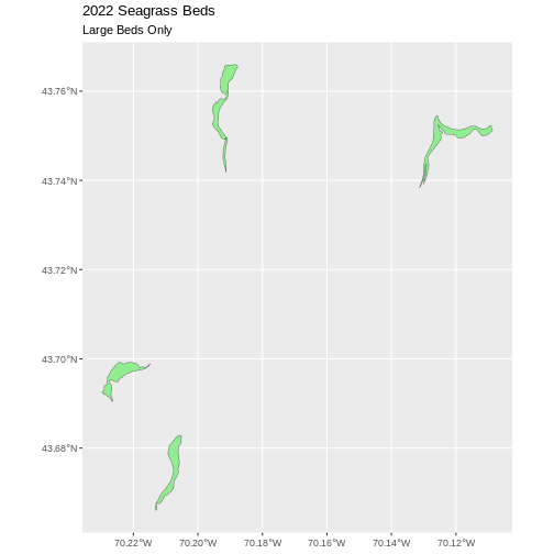
[1] 4Our subsetting operation reduces the features count 4
93. This means that 4 polygons in our spatial object are larger than 25
Hectares. We can plot only these big beds
R
ggplot() +
  geom_sf(data = large_beds, fill = "lightgreen") +
  ggtitle("2022 Seagrass Beds", subtitle = "Large Beds Only") +
  coord_sf()
There are four features in our large beds subset. But we don’t have
any more information than that they are large. Let’s adjust the colors
used in our plot. If we have 4 features in our vector object, we can
plot each using a unique color by assigning a column name to the color
aesthetic (fill =). We use the syntax
aes(fill = ) to do this. Let’s look at
Cover_Pct to differentiate sparse from dense beds.
R
ggplot() +
  geom_sf(data = large_beds, aes(fill = Cover_Pct)) +
  labs(color = 'Percent Cover of Seagrass') +
  ggtitle("2022 Seagrass Beds", subtitle = "Sparse Beds Only") +
  coord_sf()
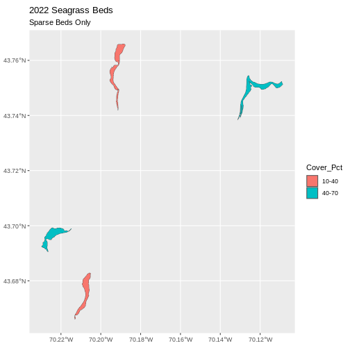
Now, we see that there are in some dense and some sparse beds that are big.
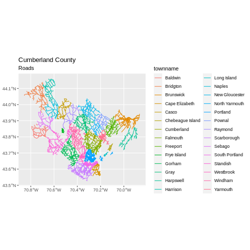
First we will save an object with only the roads in Cumberland:
R
cumberland_roads <- roads_maine %>%
  filter(cntyname == "Cumberland")
Let’s check how many features there are in this subset:
R
nrow(cumberland_roads)
OUTPUT
[1] 18246Now let’s plot that data:
R
ggplot() +
  geom_sf(data = cumberland_roads,
          aes(color = townname),
          size = 1.5) +
  ggtitle("Cumberland County", subtitle = "Roads") +
  coord_sf()
Challenge: Subset Spatial Polygon Objects and Plotting
Are dense beds large or small? From seagrass_casco_2022,
subset out only the dense beds - Cover_Pct == "70-100".
How many dense beds are there?
What is the distribution of their size?
Plotthem . To make it interesting, set the color (not the fill) to map to
Hectaresso that we can see where big dense beds exist. To further assist with this A) you will need to setlinewidth = 2, as otherwise you won’t be able to see the beds well and B) you’ll need to use a binned color scale, like we did with rasters. I’m a fan ofscale_color_viridis_b()here, but also feel free to try some options fromscale_color_fermenter()or play with then.binsargument.
- First we will save an object with only the stone wall lines and check the number of features:
R
dense_beds <- seagrass_casco_2022 %>%
  filter(Cover_Pct == "70-100")

nrow(dense_beds)
OUTPUT
[1] 79- Is the distribution different than the size of all beds? Let’s see.
R
ggplot(data = dense_beds,
       aes(x = Hectares)) +
  geom_histogram(bins = 50)
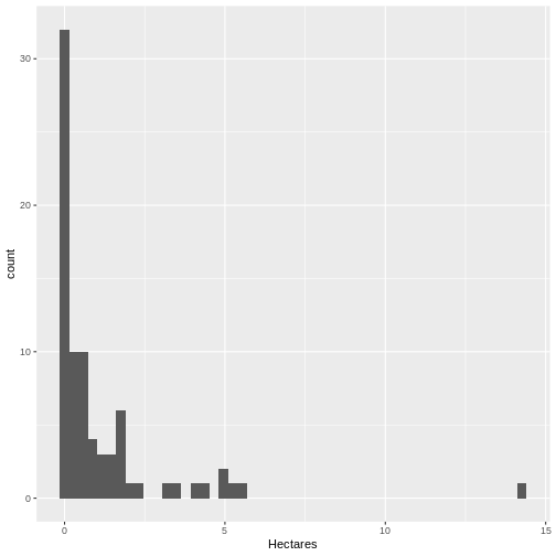
It’s roughly similar, although there seem to be more mid-size beds.
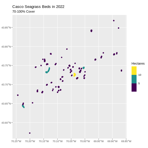
- Last, we can plot the data:
R
ggplot() +
  geom_sf(data = dense_beds, aes(color = Hectares),
          linewidth = 2) +
  ggtitle("Casco Seagrass Beds in 2022", subtitle = "70-100% Cover") +
  coord_sf() +
  scale_color_viridis_b()
Customize Plots
In the examples above, ggplot() automatically selected
colors for each line based on a default color order. If we don’t like
those default colors, we can create a vector of colors - one for each
feature.
First we will check how many unique levels our factor has:
R
unique(seagrass_casco_2022$Cover_Pct)
OUTPUT
[1] "0-10" "40-70" "70-100" "10-40" Then we can create a palette of four colors, one for each feature in our vector object.
R
bed_colors <- c("blue", "purple", "lightgreen", "orange")
We can tell ggplot to use these colors when we plot the
data.
R
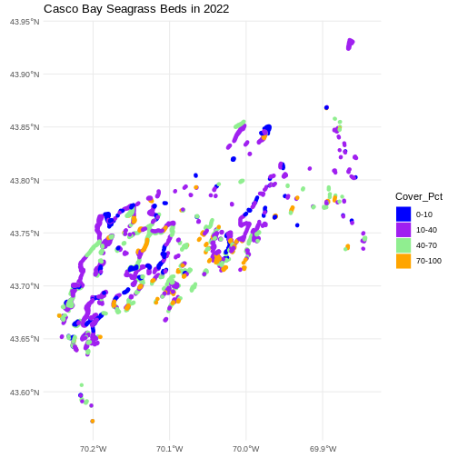
ggplot() +
  geom_sf(data = seagrass_casco_2022,
          aes(color = Cover_Pct, fill = Cover_Pct),
          linewidth = 2) +
  scale_color_manual(values = bed_colors) +
  scale_fill_manual(values = bed_colors) +
  ggtitle("Casco Bay Seagrass Beds in 2022") +
  coord_sf() +
  theme_minimal()
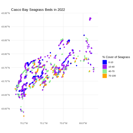
Improve Our Plot Legend
Let’s improve the legend of our plot. We’ve already created a
legenend for Cover_Pct by default. Let’s start by making
the title be readable using labs() to give it titles. Note,
color and fill must have the same title, otherwise the legend
splits.
R
ggplot() +
  geom_sf(data = seagrass_casco_2022,
          aes(color = Cover_Pct, fill = Cover_Pct),
          linewidth = 2) +
  scale_color_manual(values = bed_colors) +
  scale_fill_manual(values = bed_colors) +
  labs(color = '% Cover of Seagrass', fill = "% Cover of Seagrass") +
  ggtitle("Casco Bay Seagrass Beds in 2022") +
  coord_sf() +
  theme_minimal()
We can change the appearance of our legend by manually setting
different parameters using the theme() function.
-
legend.title: change the legend title font size -
legend.text: change the legend text font size -
legend.box.background: add an outline box -
legend.position: where you want the legend. Options include “none”, “left”, “right”, “bottom”, “top”, or two-element numeric vector.
Note, some of these will need an element_*() function.
To dig deep deep into plot customization, see ?theme
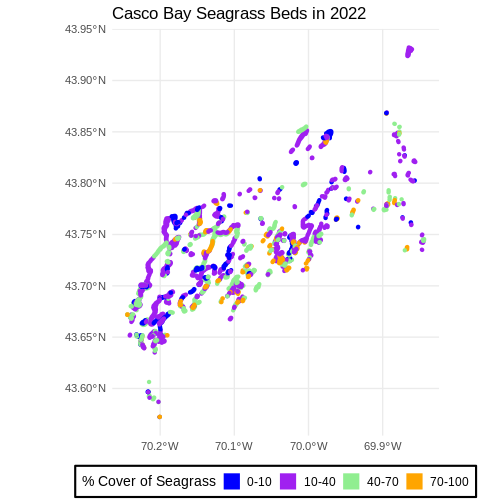
R
ggplot() +
  geom_sf(data = seagrass_casco_2022,
          aes(color = Cover_Pct, fill = Cover_Pct),
          linewidth = 2) +
  scale_color_manual(values = bed_colors) +
  scale_fill_manual(values = bed_colors) +
  labs(color = '% Cover of Seagrass', fill = "% Cover of Seagrass") +
  ggtitle("Casco Bay Seagrass Beds in 2022") +
  coord_sf() +
  theme_minimal(base_size = 14)  +
  theme(legend.title = element_text(size = 14),
        legend.text = element_text(size = 12),
        legend.box.background = element_rect(linewidth = 1),
        legend.position = "bottom")
theme_minimal() here is a premade ggplot2 theme. You can
also use theme() to make your own customized themes.
Challenge: Visualizing Change
Create a similar plot from the 2023 data. There are some differences.
Cover_Pct is slightly different. You’ll have to filter out
the "0%“` beds in order to use the identical color palette
(a good idea in order to see change).
Do you see differences between 2013 and 2022?
First we explore load and filter the data.
R
seagrass_casco_2013 <-
  st_read("data/maine_gov_seagrass/MaineDEP_Casco_Bay_Eelgrass_2013/") |>
  filter(Cover_Pct != "0%")
OUTPUT
Reading layer `MaineDEP_Casco_Bay_Eelgrass_2013' from data source
  `/home/runner/work/r-raster-vector-geospatial/r-raster-vector-geospatial/site/built/data/maine_gov_seagrass/MaineDEP_Casco_Bay_Eelgrass_2013'
  using driver `ESRI Shapefile'
Simple feature collection with 1056 features and 7 fields
Geometry type: POLYGON
Dimension:     XY
Bounding box:  xmin: -70.2477 ymin: 43.5896 xmax: -69.84402 ymax: 43.93288
Geodetic CRS:  WGS 84
Then, honestly, we can re-use the same plotting code as above.
R
ggplot() +
  geom_sf(data = seagrass_casco_2013,
          aes(color = Cover_Pct, fill = Cover_Pct),
          linewidth = 2) +
  scale_color_manual(values = bed_colors) +
  scale_fill_manual(values = bed_colors) +
  labs(color = '% Cover of Seagrass', fill = "% Cover of Seagrass",
       title = "Casco Bay Seagrass Beds in 2013") +
  coord_sf() +
  theme_minimal(base_size = 14)  +
  theme(legend.title = element_text(size = 14),
        legend.text = element_text(size = 12),
        legend.box.background = element_rect(linewidth = 1),
        legend.position = "bottom")
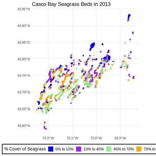
Flip back and forth between the two maps. Qualitatively, it looks like beds are less dense.
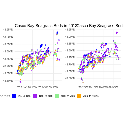
Data Tip
You can plot multiple plot panels next to each other using the patchwork library.
R
library(patchwork)

beds_2013 <- ggplot() +
  geom_sf(data = seagrass_casco_2013,
          aes(color = Cover_Pct, fill = Cover_Pct),
          linewidth = 2) +
  scale_color_manual(values = bed_colors) +
  scale_fill_manual(values = bed_colors) +
  labs(color = '% Cover of Seagrass', fill = "% Cover of Seagrass",
       title = "Casco Bay Seagrass Beds in 2013") +
  coord_sf() +
  theme_minimal(base_size = 14)

beds_2022 <- ggplot() +
  geom_sf(data = seagrass_casco_2022,
          aes(color = Cover_Pct, fill = Cover_Pct),
          linewidth = 2) +
  scale_color_manual(values = bed_colors) +
  scale_fill_manual(values = bed_colors) +
  labs(title = "Casco Bay Seagrass Beds in 2022") +
  coord_sf() +
  theme_minimal(base_size = 14)

# the patchwork - note removing one legend for ease of viz
# as they are the same but different text
(beds_2013 & theme(legend.position = 'bottom')) +
  (beds_2022 & theme(legend.position = "none"))