Convert from .csv to a Vector Layer
Last updated on 2024-03-12 | Edit this page
WARNING
Warning in
download.file("https://www.naturalearthdata.com/http//www.naturalearthdata.com/download/110m/physical/ne_110m_graticules_all.zip",
: cannot open URL
'https://www.naturalearthdata.com/http//www.naturalearthdata.com/download/110m/physical/ne_110m_graticules_all.zip':
HTTP status was '500 Internal Server Error'
ERROR
Error in download.file("https://www.naturalearthdata.com/http//www.naturalearthdata.com/download/110m/physical/ne_110m_graticules_all.zip", : cannot open URL 'https://www.naturalearthdata.com/http//www.naturalearthdata.com/download/110m/physical/ne_110m_graticules_all.zip'Overview
Questions
- How can I import CSV files as vector layers in R?
Objectives
- Import .csv files containing x,y coordinate locations into R as a data frame.
- Convert a data frame to a spatial object.
- Export a spatial object to a text file.
Things You’ll Need To Complete This Episode
See the lesson homepage for detailed information about the software, data, and other prerequisites you will need to work through the examples in this episode.
You’ll need to load the following libraries
R
library(ggplot2)
library(dplyr)
library(sf)
This episode will review how to import spatial points stored in
.csv (Comma Separated Value) format into R as an
sf spatial object. We will also plot it and save the data
as an ESRI shapefile.
Spatial Data in Text Format
In the Intro to R for
Geospatial lessons, we worked with data from Maine
DMR urchin surves and Steneck/Rasher lab surveys of kelp forests up
and down the coast of Maine. This data contains x, y
(point) locations for study sites in the form of the variables
longitude and latitude.
We would like to:
- Create a map of these site locations.
- Create a map showing the coastline as a reference
- Export the data in an ESRI
shapefileformat to share with our colleagues. Thisshapefilecan be imported into most GIS software.
Spatial data are sometimes stored in a text file format
(.txt or .csv). If the text file has an
associated x and y location column, then we
can convert it into an sf spatial object. The
sf object allows us to store both the x,y
values that represent the coordinate location of each point and the
associated attribute data - or columns describing each feature in the
spatial object.
Import .csv
To begin let’s import a .csv file that contains site
coordinate locations from these subtidal locations and look at the
structure of that new object:
R
dmr <-
  read.csv("data/maine_dmr/dmr_kelp_urchin.csv")

str(dmr)
OUTPUT
'data.frame':	1478 obs. of  15 variables:
 $ year         : int  2001 2001 2001 2001 2001 2001 2001 2001 2001 2001 ...
 $ region       : chr  "York" "York" "York" "York" ...
 $ exposure.code: int  4 4 4 4 4 2 2 3 2 2 ...
 $ coastal.code : int  3 3 3 4 3 2 2 3 2 2 ...
 $ latitude     : num  43.1 43.3 43.4 43.5 43.5 ...
 $ longitude    : num  -70.7 -70.6 -70.4 -70.3 -70.3 ...
 $ depth        : int  5 5 5 5 5 5 5 5 5 5 ...
 $ crust        : num  60 75.5 73.5 63.5 72.5 6.1 31.5 31.5 40.5 53 ...
 $ understory   : num  100 100 80 82 69 38.5 74 96.5 60 59.5 ...
 $ kelp         : num  1.9 0 18.5 0.6 63.5 92.5 59 7.7 52.5 29.2 ...
 $ urchin       : num  0 0 0 0 0 0 0 0 0 0 ...
 $ month        : int  6 6 6 6 6 6 6 6 6 6 ...
 $ day          : int  13 13 14 14 14 15 15 15 8 8 ...
 $ survey       : chr  "dmr" "dmr" "dmr" "dmr" ...
 $ site         : int  42 47 56 61 62 66 71 70 23 22 ...
We now have a data frame that contains 1478 locations (rows) and 15
variables (attributes). Note that all of our character data was imported
into R as character (text) data. Next, let’s explore the dataframe to
determine whether it contains columns with coordinate values. If we are
lucky, our .csv will contain columns labeled:
- “X” and “Y” OR
- Latitude and Longitude OR
- easting and northing (UTM coordinates)
Let’s check out the column names of our dataframe.
R
names(dmr)
OUTPUT
 [1] "year"          "region"        "exposure.code" "coastal.code"
 [5] "latitude"      "longitude"     "depth"         "crust"
 [9] "understory"    "kelp"          "urchin"        "month"
[13] "day"           "survey"        "site"
Identify X,Y Location Columns
Our column names include several fields that might contain spatial
information. The dmr$longitude and
dmr$latitude columns contain coordinate values. We can
confirm this by looking at the first six rows of our data.
R
head(dmr$longitude)
OUTPUT
[1] -70.66749 -70.55645 -70.38046 -70.32038 -70.30401 -70.10721R
head(dmr$latitude)
OUTPUT
[1] 43.06709 43.28014 43.40849 43.50783 43.52791 43.72766We have coordinate values in our data frame. In order to convert our
data frame to an sf object, we also need to know the CRS
associated with those coordinate values.
There are several ways to figure out the CRS of spatial data in text format.
- We can check the file metadata in hopes that the CRS was recorded in the data.
- We can explore the file itself to see if CRS information is embedded in the file header or somewhere in the data columns.
In our case, as we have decimal degrees, this is likely a standard WGS 84 defined under EPSG code 4326. However, it always behoves you to check!
If we had had columns like easting and
northing columns, then we are likely dealing with UTM or
otherwise. Check if there is a geodeticDatum and a
utmZone column. These appear to contain CRS information
(datum and projection). Or, again, check the
metadata for the data set.
In When Vector Data
Don’t Line Up - Handling Spatial Projection & CRS in R we
learned about the components of a proj4 string and
EPSG. We have everything we need to assign a CRS to our
data frame. If we wanted, we could use another loaded shapefile to
extract a CRS and use it here. That is not needed, however, as
sf lets us use EPSG codes.
.csv to sf object
Let’s convert our dataframe into an sf object. To do
this, we need to specify:
- The columns containing X (
longitude) and Y (latitude) coordinate values - The CRS. Either as an object or an EPSG code.
We will use the st_as_sf() function to perform the
conversion.
R
dmr_sf <- st_as_sf(dmr,
                   coords = c("longitude", "latitude"),
                   crs = 4326)
We should double check the CRS to make sure it is correct.
R
st_crs(dmr_sf)
OUTPUT
Coordinate Reference System:
  User input: EPSG:4326
  wkt:
GEOGCRS["WGS 84",
    ENSEMBLE["World Geodetic System 1984 ensemble",
        MEMBER["World Geodetic System 1984 (Transit)"],
        MEMBER["World Geodetic System 1984 (G730)"],
        MEMBER["World Geodetic System 1984 (G873)"],
        MEMBER["World Geodetic System 1984 (G1150)"],
        MEMBER["World Geodetic System 1984 (G1674)"],
        MEMBER["World Geodetic System 1984 (G1762)"],
        MEMBER["World Geodetic System 1984 (G2139)"],
        ELLIPSOID["WGS 84",6378137,298.257223563,
            LENGTHUNIT["metre",1]],
        ENSEMBLEACCURACY[2.0]],
    PRIMEM["Greenwich",0,
        ANGLEUNIT["degree",0.0174532925199433]],
    CS[ellipsoidal,2],
        AXIS["geodetic latitude (Lat)",north,
            ORDER[1],
            ANGLEUNIT["degree",0.0174532925199433]],
        AXIS["geodetic longitude (Lon)",east,
            ORDER[2],
            ANGLEUNIT["degree",0.0174532925199433]],
    USAGE[
        SCOPE["Horizontal component of 3D system."],
        AREA["World."],
        BBOX[-90,-180,90,180]],
    ID["EPSG",4326]]
Plot Spatial Object
We now have a spatial R object, we can plot our newly created spatial object.
R
ggplot() +
  geom_sf(data = dmr_sf,
          mapping = aes(color = region)) +
  ggtitle("Map of Site Locations")
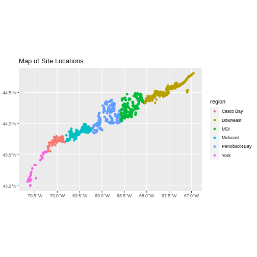
Looks good! If we really want to check, we can either load up our
state of Maine shapefile or plot it against a tiles with
leaflet.
R
library(leaflet)

pal <- colorFactor("Set1",
                   domain = dmr_sf$region)

leaflet() |>
  addTiles() |>
  addCircles(data = dmr_sf,
             color = ~pal(region))
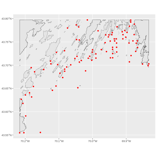
R
# Load Casco
casco_dmr <- read.csv(
  "data/maine_dmr/casco_kelp_urchin.csv"
)


# Turn it into an sf object
casco_dmr_sf <- st_as_sf(casco_dmr,
                         coords = c("longitude", "latitude"),
                         crs = 4326)

# Load Maine
maine <- st_read(
  "data/maine_gov_maps/Maine_State_Boundary_Polygon_Feature/Maine_State_Boundary_Polygon_Feature.shp",
  quiet = TRUE)

# Crop to Casco
casco <- st_crop(maine |> st_make_valid(),
                 casco_dmr_sf)

# Plot!
ggplot() +
  geom_sf(data = casco) +
  geom_sf(data = casco_dmr_sf, color = "red")
Key Points
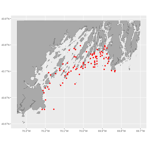
Sometimes, we want to crop to a larger area than just the data set.
For that, we can create a box from the extent of the new vector object
using st_bbox(). This, though, is really just a vector, so
we need to turn it into a polygon using st_sfc() (sfc
objects are just a raw shape, while sf contains data).
To make this box bigger, we can use st_buffer() which
will create a buffer area using a distance specified in meters. So,
1e4 would be 10km.
This technique can be a nice way to put a new vector file in context, as follows.
R
#Make a bounding box of the Casco Bay area from the data
casco_bbox <- st_bbox(casco_dmr_sf) |>
  st_as_sfc()

# Enlarge it by 10 km
casco_bbox_big <- st_buffer(casco_bbox,
                            dist = 1e4)

# Crop to the new area
casco <- st_crop(maine |> st_make_valid(),
                 casco_bbox_big)

# Plot!
ggplot() +
  geom_sf(data = casco, fill = "darkgrey") +
  geom_sf(data = casco_dmr_sf, color = "red")
Export to an ESRI shapefile
We can write an R spatial object to an ESRI shapefile
using the st_write function in sf. To do this
we need the following arguments:
- the name of the spatial object (
dmr_sf) - the directory where we want to save our ESRI
shapefile(to usecurrent = getwd()or you can specify a different path). You can also usedir.create()no make a new directory. - the name of the new ESRI
shapefile(dmr_kelp_urchins) - the driver which specifies the file format (ESRI Shapefile)
We can now export the spatial object as an ESRI
shapefile. Note - this will make a few files.
R
dir.create("data/dmr_kelp_urchins")
st_write(dmr_sf,
         "data/dmr_kelp_urchins/dmr_kelp_urchins.shp", driver = "ESRI Shapefile")