Extracting Data from Rasters using Vectors
Last updated on 2024-03-12 | Edit this page
WARNING
Warning in
download.file("https://www.naturalearthdata.com/http//www.naturalearthdata.com/download/110m/physical/ne_110m_graticules_all.zip",
: cannot open URL
'https://www.naturalearthdata.com/http//www.naturalearthdata.com/download/110m/physical/ne_110m_graticules_all.zip':
HTTP status was '500 Internal Server Error'
ERROR
Error in download.file("https://www.naturalearthdata.com/http//www.naturalearthdata.com/download/110m/physical/ne_110m_graticules_all.zip", : cannot open URL 'https://www.naturalearthdata.com/http//www.naturalearthdata.com/download/110m/physical/ne_110m_graticules_all.zip'Overview
Questions
- How can I crop raster objects to vector objects, and extract the summary of raster pixels?
Objectives
- Crop a raster to the extent of a vector layer.
- Extract values from a raster that correspond to a vector file overlay.
Things You’ll Need To Complete This Episode
See the lesson homepage for detailed information about the software, data, and other prerequisites you will need to work through the examples in this episode.
Load Libraries
This episode explains how to crop a raster using the extent of a vector layer. We will also cover how to extract values from a raster that occur within a set of polygons, or in a buffer (surrounding) region around a set of points.
R
library(sf)
library(terra)
library(ggplot2)
library(tidyterra)
Crop a Raster to Vector Extent
We often work with spatial layers that have different spatial extents. The spatial extent of a vector layer or R spatial object represents the geographic “edge” or location that is the furthest north, south east and west. Thus it represents the overall geographic coverage of the spatial object.
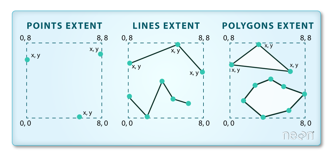 Image Source: National Ecological
Observatory Network (NEON)
Image Source: National Ecological
Observatory Network (NEON)
The graphic below illustrates the extent of several of the spatial layers that we have worked with in this workshop and one new one:
- Area of interest (AOI) – blue
- Seagrass Beds – purple
- Areas surveyed for kelp and urchins (marked with white dots)– black
- Water turbidity in GeoTIFF format – green
R
# Casco AOI
aoi_boundary_casco <- st_read(
  "data/maine_gov_maps/casco_aoi/casco_bay_aoi.shp")

# seagrass in 2022
seagrass_casco_2022 <- st_read(
  "data/maine_gov_seagrass/MaineDEP_Casco_Bay_Seagrass_2022/MaineDEP_Casco_Bay_Seagrass_2022.shp")

# subtidal samples
dmr_casco <-
  read.csv("data/maine_dmr/casco_kelp_urchin.csv") |>
  st_as_sf(coords = c("longitude", "latitude"), crs = 4326)

# turbidity from modis
turbidity_modis <- rast("data/modis/GIOVANNI-g4.timeAvgMap.MODISA_L3m_KD_Mo_4km_R2022_0_Kd_490.20230701-20230930.71W_42N_66W_45N.tif")
Frequent use cases of cropping a raster file include reducing file size and creating maps. Sometimes we have a raster file that is much larger than our study area or area of interest. It is often more efficient to crop the raster to the extent of our study area to reduce file sizes as we process our data. Cropping a raster can also be useful when creating pretty maps so that the raster layer matches the extent of the desired vector layers.
Crop a Raster Using Vector Extent
We can use the crop() function to crop a raster to the
extent of another spatial object. To do this, we need to specify the
raster to be cropped and the spatial object that will be used to crop
the raster. R will use the extent of the spatial object as
the cropping boundary.
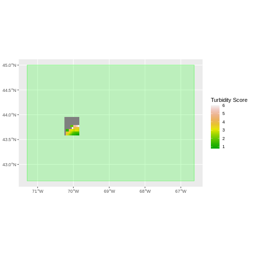
To illustrate this, we will crop the MODIS turbidity data to only
include the area of interest (AOI). Let’s start by plotting the full
extent of the CHM data and overlay where the AOI falls within it. The
boundaries of the AOI will be colored blue, and we use
fill = NA to make the area transparent.
R
ggplot() +
  geom_spatraster(data = turbidity_modis) +
  scale_fill_gradientn(name = "Turbidity Score", colors = terrain.colors(10)) +
  geom_sf(data = aoi_boundary_casco, color = "blue", fill = NA) +
  coord_sf()
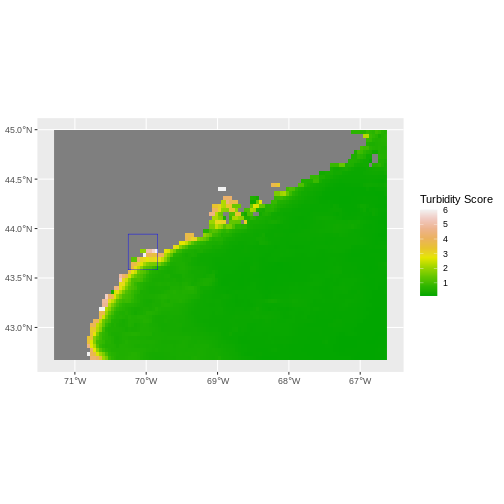
Now that we have visualized the area of the turbidity data we want to
subset, we can perform the cropping operation. We are going to
crop() function from the raster package to create a new
object with only the portion of the MODIS data that falls within the
boundaries of the AOI.
R
turbidity_casco <- crop(x = turbidity_modis, y = aoi_boundary_casco)
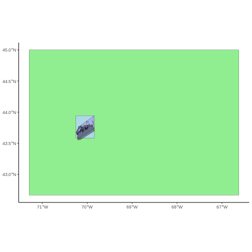
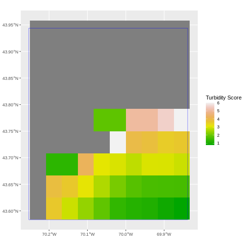
Now we can plot the cropped MODIS data, along with a boundary box
showing the full MODIS extent. However, remember, since this is raster
data, we need to convert to a data frame in order to plot using
ggplot. To get the boundary box from MODIS, the
st_bbox() will extract the 4 corners of the rectangle that
encompass all the features contained in this object. The
st_as_sfc() converts these 4 coordinates into a polygon
that we can plot:
R
ggplot() +
  geom_sf(data = st_as_sfc(st_bbox(turbidity_modis)), fill = "green",
          color = "green", alpha = .2) +
  geom_spatraster(data = turbidity_casco) +
  scale_fill_gradientn(name = "Turbidity Score", colors = terrain.colors(10)) +
  coord_sf()
The plot above shows that the full MODS extent (plotted in green) is
much larger than the resulting cropped raster. Our new cropped MODS now
has the same extent as the aoi_boundary_casco object that
was used as a crop extent (blue border below).
R
ggplot() +
  geom_spatraster(data = turbidity_casco) +
  geom_sf(data = aoi_boundary_casco, color = "blue", fill = NA) +
  scale_fill_gradientn(name = "Turbidity Score", colors = terrain.colors(10)) +
  coord_sf()
We can look at the extent of all of our other objects for this field site.
R
st_bbox(turbidity_modis)
OUTPUT
     xmin      ymin      xmax      ymax
-71.29166  42.66666 -66.62500  45.00000
R
st_bbox(turbidity_casco)
OUTPUT
     xmin      ymin      xmax      ymax
-70.25000  43.58333 -69.83333  43.95833
R
st_bbox(aoi_boundary_casco)
OUTPUT
    xmin     ymin     xmax     ymax
-70.2528  43.5834 -69.8387  43.9439
R
st_bbox(seagrass_casco_2022)
OUTPUT
     xmin      ymin      xmax      ymax
-70.24464  43.57213 -69.84399  43.93221
R
st_bbox(dmr_casco)
OUTPUT
     xmin      ymin      xmax      ymax
-70.21650  43.55470 -69.83280  43.79721
Our dmr_casco location extent is not the largest It
would be nice to see our vegetation plot locations plotted on top of the
turbidity information.
R
turbidity_dmr_sites <- crop(x = turbidity_modis, y = dmr_casco)

ggplot() +
  geom_spatraster(data = turbidity_dmr_sites) +
  scale_fill_gradientn(name = "Canopy Height", colors = terrain.colors(10)) +
  geom_sf(data = dmr_casco)
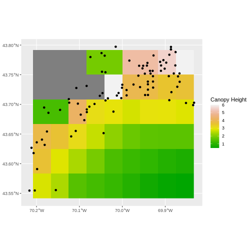
In the plot above, created in the challenge, all the site locations (black dots) appear on the turbidity raster layer except for a few. some are situated on the blank space to the left of the map. Why?
The raster data is in a resolution such that many of the coastal pixels are eliminated as not valid data. Check the resolution of the raster. It’s 0.417 degrees. 1 degree is ~ 111,111 meters. So, 1 pixel here is ~ 4,600 meters, or 4.6km. We are going to lose a lot of things close to the coast.
Thinking about data source resolution is key in thinking about rasters when you want to get data close to the coast versus more offshore.
Extract Raster Pixels Values Using Vector Polygons
Often we want to extract values from a raster layer for particular locations - for example, plot locations that we are sampling on the ground. We can extract all pixel values within 20m of our x,y point of interest. These can then be summarized into some value of interest (e.g. mean, maximum, total).
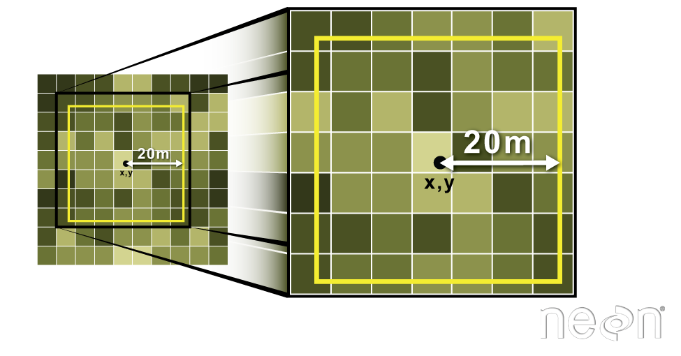 Image Source: National Ecological Observatory Network (NEON)
To do this in R, we use the extract() function. The
extract() function requires:
- The raster that we wish to extract values from,
- The vector layer containing the polygons that we wish to use as a boundary or boundaries,
- we can tell it to store the output values in a data frame using
raw = FALSE(this is optional).
We will begin by extracting all canopy height pixel values located
within our aoi_boundary_casco polygon which surrounds the
tower located at the NEON Harvard Forest field site.
R
names(turbidity_casco) <- "turbidity"

turbidity_df <- extract(x = turbidity_casco,
                     y = aoi_boundary_casco,
                     raw = FALSE)

str(turbidity_df)
OUTPUT
'data.frame':	90 obs. of  2 variables:
 $ ID       : num  1 1 1 1 1 1 1 1 1 1 ...
 $ turbidity: num  NA NA NA NA NA NA NA NA NA NA ...
When we use the extract() function, R extracts the value
for each pixel located within the boundary of the polygon being used to
perform the extraction - in this case the
aoi_boundary_casco object (a single polygon). Here, the
function extracted values from 90 pixels.
We can create a histogram of turbidity values within the boundary to
better understand the structure or height distribution of turbidity at
our site. We will use the column turbidity from our data
frame as our x values.
R
ggplot() +
  geom_histogram(data = turbidity_df, aes(x = turbidity)) +
  ggtitle("Histogram of turbidity values") +
  xlab("turbidity") +
  ylab("Frequency of Pixels")
OUTPUT
`stat_bin()` using `bins = 30`. Pick better value with `binwidth`.WARNING
Warning: Removed 52 rows containing non-finite values (`stat_bin()`).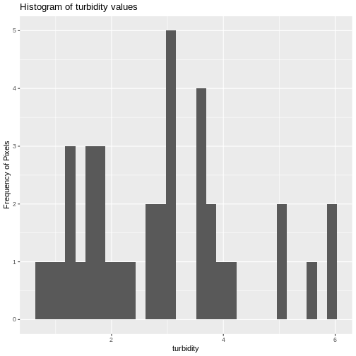
We can also use the summary() function to view
descriptive statistics including min, max, and mean height values. These
values help us better understand vegetation at our field site.
R
summary(turbidity_df$turbidity)
OUTPUT
   Min. 1st Qu.  Median    Mean 3rd Qu.    Max.    NA's
 0.7771  1.6590  2.8625  2.8668  3.6165  6.0000      52
Summarize Extracted Raster Values
We often want to extract summary values from a raster. We can tell R
the type of summary statistic we are interested in using the
fun = argument. Let’s extract a mean height value for our
AOI.
R
mean_turbidity_aoi <- extract(x = turbidity_casco,
                                 y = aoi_boundary_casco,
                                fun = mean, na.rm = TRUE)

mean_turbidity_aoi
OUTPUT
  ID turbidity
1  1  2.866811
It appears that the mean height value, extracted from our LiDAR data derived canopy height model is 22.43 meters.
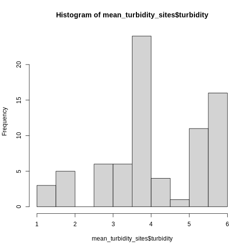
Extract Data using x,y Locations
We can also extract pixel values from a raster by defining a buffer
or area surrounding individual point locations using the
st_buffer() function. To do this we define the summary
argument (fun = mean) and the buffer distance
(dist = 20) which represents the radius of a circular
region around each point. By default, the units of the buffer are the
same units as the data’s CRS. All pixels that are touched by the buffer
region are included in the extract.
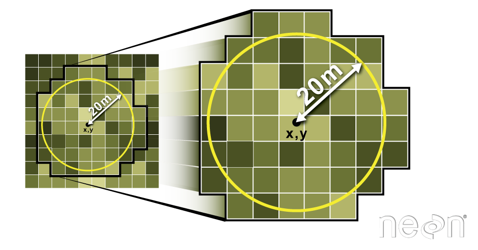 Image Source: National Ecological Observatory Network (NEON)
Let’s put this into practice by figuring out the mean tree height in
the 20m around the tower location (point_HARV).
R
mean_turbidity_sites <- extract(x = turbidity_casco,
                                  y = st_buffer(dmr_casco, dist = 20),
                                  fun = mean,
                                raw = FALSE)

hist(mean_turbidity_sites$turbidity)
Challenge: Extract Temperature Values For Seagrass Beds
You can also extract data from polygons. Let’s look at temperature in seagrass beds in 2022.
Load up “data/landsat_casco/b10_cropped/LC08_L2SP_011030_20220909_20220914_02_T1_ST_B10.TIF”. Reproject it and crop it to the extent of
seagrass_casco_2022- smaller rasters = faster extraction.Extract the average SST in each bed.
cbind()it back toseagrass_casco_2022Plot SST by Hectares of seagrass bed.
- We can do this as a processing chain!
R
sst <- rast(
  "data/landsat_casco/b10_cropped/LC08_L2SP_011030_20220909_20220914_02_T1_ST_B10.TIF"
  ) |>
  project(crs(seagrass_casco_2022)) |>
  crop(seagrass_casco_2022)
- We can extract now. Note, some beds will throw an NaN, as
R
temp_beds <- extract(sst,
                     seagrass_casco_2022,
                     fun = mean,
                     na.rm = TRUE,
                     raw = FALSE)

seagrass_casco_2022 <- cbind(seagrass_casco_2022, temp_beds)
- It’s just a
geom_point()
R
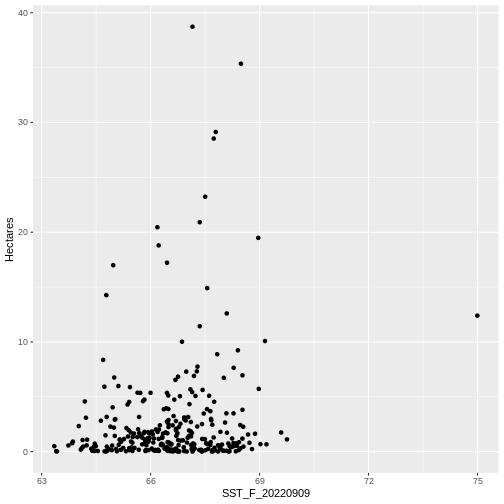
ggplot(data = seagrass_casco_2022) +
  geom_point(aes(x = SST_F_20220909, y = Hectares))
WARNING
Warning: Removed 314 rows containing missing values (`geom_point()`).