Intro to Raster Data
- The GeoTIFF file format includes metadata about the raster data.
- To plot raster data with the
ggplot2package, we need to convert it to a dataframe. - R stores CRS information in the Proj4 format.
- Be careful when dealing with missing or bad data values.
Plot Raster Data
- Continuous data ranges can be grouped into categories using
mutate()andcut()or with a binned color scale inggplot2. - Use built-in color palettes with
scale_fill_viridis_borscale_fill_fermenter()or set your preferred color scheme manually. - Interactive plotting with
plet()and theleafletlibrary can lead to even better insights as you zoom in and out.
Open and Plot Vector Layers
- Metadata for vector layers include geometry type, CRS, and extent.
- Load spatial objects into R with the
st_read()function. - Spatial objects can be plotted directly with
ggplotusing thegeom_sf()function. No need to convert to a dataframe.
Explore and Plot by Vector Layer Attributes
- Spatial objects in
sfare similar to standard data frames and can be manipulated using the same functions. - Almost any feature of a plot can be customized using the various
functions and options in the
ggplot2package.
Plot Multiple Vector Layers
- Use the
+operator to add multiple layers to a ggplot. - Use
st_crop()to put spatially subset a vector data set. - Multi-layered plots can combine multiple vector data sets.
- Use
leafletor zooming inggplot2to see small spatial features.
Handling Spatial Projection & CRS
- Multi-layered plots can combine vector and raster data sets.
-
ggplot2automatically converts all objects in a plot to the same CRS. - Still be aware of the CRS and extent for each object.
-
project()andst_transform()will reproject raster and vector data. -
crop()andst_crop()will crop raster and vector data.
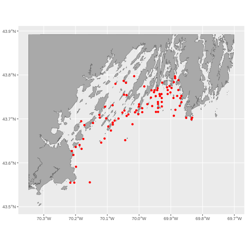
Convert from .csv to a Vector Layer
Sometimes, we want to crop to a larger area than just the data set.
For that, we can create a box from the extent of the new vector object
using st_bbox(). This, though, is really just a vector, so
we need to turn it into a polygon using st_sfc() (sfc
objects are just a raw shape, while sf contains data).
To make this box bigger, we can use st_buffer() which
will create a buffer area using a distance specified in meters. So,
1e4 would be 10km.
This technique can be a nice way to put a new vector file in context, as follows.
R
#Make a bounding box of the Casco Bay area from the data
casco_bbox <- st_bbox(casco_dmr_sf) |>
  st_as_sfc()

# Enlarge it by 10 km
casco_bbox_big <- st_buffer(casco_bbox,
                            dist = 1e4)

# Crop to the new area
casco <- st_crop(maine |> st_make_valid(),
                 casco_bbox_big)

# Plot!
ggplot() +
  geom_sf(data = casco, fill = "darkgrey") +
  geom_sf(data = casco_dmr_sf, color = "red")
- Know the projection (if any) of your point data prior to converting to a spatial object.
- Convert a data frame to an
sfobject using thest_as_sf()function. - Export an
sfobject as text using thest_write()function.
Extracting Data from Rasters using Vectors
- Use the
crop()function to crop a raster object. - Use the
extract()function to extract pixels from a raster object that fall within a particular extent boundary. - Use the
ext()function to define an extent.
Work with Multi-Band Rasters
- A single raster file can contain multiple bands or layers.
- Use the
rast()function to load all bands in a multi-layer raster file into R. - Individual bands within a SpatRaster can be accessed, analyzed, and visualized using the same functions no matter how many bands it holds.
Raster Calculations
- Rasters can be computed on using mathematical functions.
- The
lapp()andapp()function provides an efficient way to do raster math. - The
writeRaster()function can be used to write raster data to a file.