Open and Plot Vector Layers
Last updated on 2024-03-12 | Edit this page
WARNING
Warning in
download.file("https://www.naturalearthdata.com/http//www.naturalearthdata.com/download/110m/physical/ne_110m_graticules_all.zip",
: cannot open URL
'https://www.naturalearthdata.com/http//www.naturalearthdata.com/download/110m/physical/ne_110m_graticules_all.zip':
HTTP status was '500 Internal Server Error'
ERROR
Error in download.file("https://www.naturalearthdata.com/http//www.naturalearthdata.com/download/110m/physical/ne_110m_graticules_all.zip", : cannot open URL 'https://www.naturalearthdata.com/http//www.naturalearthdata.com/download/110m/physical/ne_110m_graticules_all.zip'Overview
Questions
- How can I distinguish between and visualize point, line and polygon vector data?
Objectives
- Know the difference between point, line, and polygon vector elements.
- Load point, line, and polygon vector layers into R.
- Access the attributes of a spatial object in R.
First, some libraries you might not have loaded at the moment.
R
library(terra)
library(ggplot2)
library(dplyr)
library(sf)
Things You’ll Need To Complete This Episode
See the lesson homepage for detailed information about the software, data, and other prerequisites you will need to work through the examples in this episode.
Starting with this episode, we will be moving from working with
raster data to working with vector data. In this episode, we will open
and plot point, line and polygon vector data loaded from ESRI’s
shapefile format into R. These data refer to data from the
Maine GeoLibrary
Data Catalogue on seagrass beds, public roads, and boat launches. In
later episodes, we will learn how to work with raster and vector data
together and combine them into a single plot.
Import Vector Data
We will use the sf package to work with vector data in
R. We will also use the terra package, which has been
loaded in previous episodes, so we can explore raster and vector spatial
metadata using similar commands. Make sure you have the sf
library loaded.
R
library(sf)
The vector layers that we will import from ESRI’s
shapefile format are:
- A polygon vector layer representing our field site boundary,
- A line vector layer representing the public roads of Maine, and
- A point vector layer representing the location of the boat launches around Maine.
The first vector layer that we will open contains the boundary of our
study area (or our Area Of Interest or AOI, hence the name
aoiBoundary). To import a vector layer from an ESRI
shapefile we use the sf function
st_read(). st_read() requires the file path to
the ESRI shapefile.
Let’s import our AOI:
R
aoi_boundary_casco <- st_read(
  "data/maine_gov_maps/casco_aoi/casco_bay_aoi.shp")
OUTPUT
Reading layer `casco_bay_aoi' from data source
  `/home/runner/work/r-raster-vector-geospatial/r-raster-vector-geospatial/site/built/data/maine_gov_maps/casco_aoi/casco_bay_aoi.shp'
  using driver `ESRI Shapefile'
Simple feature collection with 1 feature and 1 field
Geometry type: POLYGON
Dimension:     XY
Bounding box:  xmin: -70.2528 ymin: 43.5834 xmax: -69.8387 ymax: 43.9439
Geodetic CRS:  WGS 84
Vector Layer Metadata & Attributes
When we import the casco_bay_aoi.shp vector layer from
an ESRI shapefile into R (as our
aoi_boundary_casco object), the st_read()
function automatically stores information about the data. We are
particularly interested in the geospatial metadata, describing the
format, CRS, extent, and other components of the vector data, and the
attributes which describe properties associated with each individual
vector object.
Data Tip
The Explore and Plot by Vector Layer Attributes episode provides more information on both metadata and attributes and using attributes to subset and plot data.
Spatial Metadata
Key metadata for all vector layers includes:
- Object Type: the class of the imported object.
- Coordinate Reference System (CRS): the projection of the data.
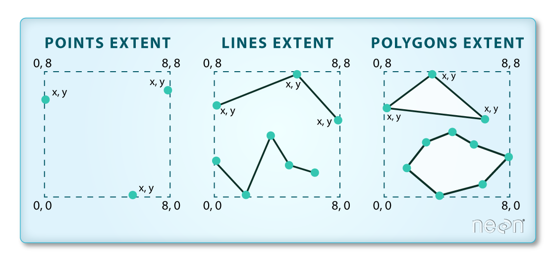
- Extent: the spatial extent (i.e. geographic area that the vector layer covers) of the data. Note that the spatial extent for a vector layer represents the combined extent for all individual objects in the vector layer.
We can view metadata of a vector layer using the
st_geometry_type(), st_crs() and
st_bbox() functions. First, let’s view the geometry type
for our AOI vector layer:
R
st_geometry_type(aoi_boundary_casco)
OUTPUT
[1] POLYGON
18 Levels: GEOMETRY POINT LINESTRING POLYGON MULTIPOINT ... TRIANGLE
Our aoi_boundary_casco is a polygon spatial object. The
18 levels shown below our output list the possible categories of the
geometry type. Now let’s check what CRS this file data is in:
R
st_crs(aoi_boundary_casco)
OUTPUT
Coordinate Reference System:
  User input: WGS 84
  wkt:
GEOGCRS["WGS 84",
    DATUM["World Geodetic System 1984",
        ELLIPSOID["WGS 84",6378137,298.257223563,
            LENGTHUNIT["metre",1]]],
    PRIMEM["Greenwich",0,
        ANGLEUNIT["degree",0.0174532925199433]],
    CS[ellipsoidal,2],
        AXIS["latitude",north,
            ORDER[1],
            ANGLEUNIT["degree",0.0174532925199433]],
        AXIS["longitude",east,
            ORDER[2],
            ANGLEUNIT["degree",0.0174532925199433]],
    ID["EPSG",4326]]
Our data in the CRS WGS 84 (it is EPSG code 4326).
The CRS is critical to interpreting the spatial object’s extent values
as it specifies units. To find the extent of our AOI, we can use the
st_bbox() function:
R
st_bbox(aoi_boundary_casco)
OUTPUT
    xmin     ymin     xmax     ymax
-70.2528  43.5834 -69.8387  43.9439
The spatial extent of a vector layer or R spatial object represents the geographic “edge” or location that is the furthest north, south east and west. Thus it represents the overall geographic coverage of the spatial object. Image Source: National Ecological Observatory Network (NEON).
Lastly, we can view all of the metadata and attributes for this R spatial object by printing it to the screen:
R
aoi_boundary_casco
OUTPUT
Simple feature collection with 1 feature and 1 field
Geometry type: POLYGON
Dimension:     XY
Bounding box:  xmin: -70.2528 ymin: 43.5834 xmax: -69.8387 ymax: 43.9439
Geodetic CRS:  WGS 84
  FID                       geometry
1   0 POLYGON ((-70.2528 43.5834,...
Spatial Data Attributes
We introduced the idea of spatial data attributes in an earlier lesson. Now we will explore how to use spatial data attributes stored in our data to plot different features.
Plot a vector layer
Next, let’s visualize the data in our sf object using
the ggplot package. Unlike with raster data, we do not need
to convert vector data to a dataframe before plotting with
ggplot.
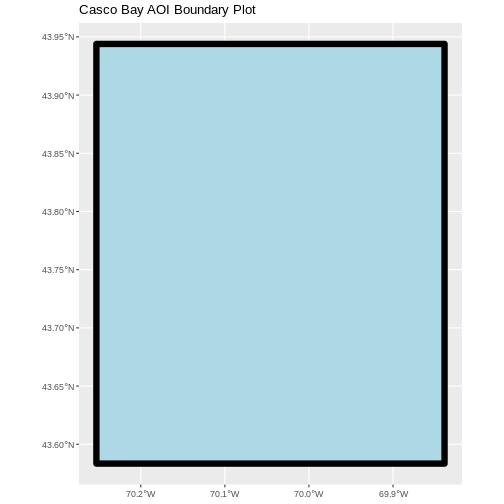
We’re going to customize our boundary plot by setting the size,
color, and fill for our plot. When plotting sf objects with
ggplot2, you need to use the coord_sf()
coordinate system.
R
ggplot() +
  geom_sf(data = aoi_boundary_casco, linewidth = 3,
          color = "black", fill = "lightblue") +
  ggtitle("Casco Bay AOI Boundary Plot") +
  coord_sf()
Challenge: Import Line and Point Vector Layers
Using the steps above, import the MaineDOT_Public_Roads and
Maine_Boat_Launches_GeoLibrary vector layers into R. Call the
MaineDOT_Public_Roads object roads_maine and the
Maine_Boat_Launches_GeoLibrary boatlaunches_maine.
Answer the following questions:
What type of R spatial object is created when you import each layer?
What is the CRS and extent for each object?
Do the files contain points, lines, or polygons?
How many spatial objects are in each file?
First we import the data:
R
roads_maine <- st_read("data/maine_gov_maps/MaineDOT_Public_Roads/MaineDOT_Public_Roads.shp")
OUTPUT
Reading layer `MaineDOT_Public_Roads' from data source
  `/home/runner/work/r-raster-vector-geospatial/r-raster-vector-geospatial/site/built/data/maine_gov_maps/MaineDOT_Public_Roads/MaineDOT_Public_Roads.shp'
  using driver `ESRI Shapefile'
Simple feature collection with 100669 features and 30 fields
Geometry type: LINESTRING
Dimension:     XY
Bounding box:  xmin: -71.04662 ymin: 43.06728 xmax: -66.95202 ymax: 47.35999
Geodetic CRS:  WGS 84
R
boatlaunches_maine <- st_read("data/maine_gov_maps/Maine_Boat_Launches_GeoLibrary/Maine_Boat_Launches_GeoLibrary.shp")
OUTPUT
Reading layer `Maine_Boat_Launches_GeoLibrary' from data source
  `/home/runner/work/r-raster-vector-geospatial/r-raster-vector-geospatial/site/built/data/maine_gov_maps/Maine_Boat_Launches_GeoLibrary/Maine_Boat_Launches_GeoLibrary.shp'
  using driver `ESRI Shapefile'
Simple feature collection with 578 features and 20 fields
Geometry type: POINT
Dimension:     XY
Bounding box:  xmin: -70.9817 ymin: 43.0859 xmax: -66.9838 ymax: 47.35484
Geodetic CRS:  WGS 84
Then we check its class:
R
class(roads_maine)
OUTPUT
[1] "sf" "data.frame"R
class(boatlaunches_maine)
OUTPUT
[1] "sf" "data.frame"We also check the CRS and extent of each object:
R
st_crs(roads_maine)
OUTPUT
Coordinate Reference System:
  User input: WGS 84
  wkt:
GEOGCRS["WGS 84",
    DATUM["World Geodetic System 1984",
        ELLIPSOID["WGS 84",6378137,298.257223563,
            LENGTHUNIT["metre",1]]],
    PRIMEM["Greenwich",0,
        ANGLEUNIT["degree",0.0174532925199433]],
    CS[ellipsoidal,2],
        AXIS["latitude",north,
            ORDER[1],
            ANGLEUNIT["degree",0.0174532925199433]],
        AXIS["longitude",east,
            ORDER[2],
            ANGLEUNIT["degree",0.0174532925199433]],
    ID["EPSG",4326]]
R
st_bbox(roads_maine)
OUTPUT
     xmin      ymin      xmax      ymax
-71.04662  43.06728 -66.95202  47.35999
R
st_crs(boatlaunches_maine)
OUTPUT
Coordinate Reference System:
  User input: WGS 84
  wkt:
GEOGCRS["WGS 84",
    DATUM["World Geodetic System 1984",
        ELLIPSOID["WGS 84",6378137,298.257223563,
            LENGTHUNIT["metre",1]]],
    PRIMEM["Greenwich",0,
        ANGLEUNIT["degree",0.0174532925199433]],
    CS[ellipsoidal,2],
        AXIS["latitude",north,
            ORDER[1],
            ANGLEUNIT["degree",0.0174532925199433]],
        AXIS["longitude",east,
            ORDER[2],
            ANGLEUNIT["degree",0.0174532925199433]],
    ID["EPSG",4326]]
R
st_bbox(boatlaunches_maine)
OUTPUT
     xmin      ymin      xmax      ymax
-70.98170  43.08590 -66.98380  47.35484
To see the number of objects in each file, we can look at the output
from when we read these objects into R. roads_maine
contains 100669 features (all lines) and boatlaunches_maine
contains 578 points.