Intro to Raster Data
Figure 1
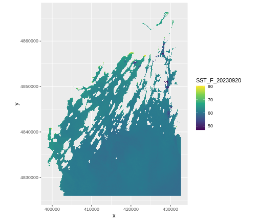
Figure 2
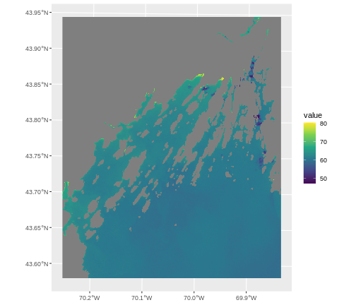
Figure 3
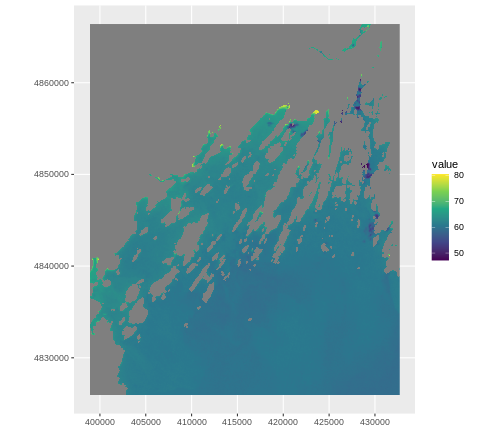
Figure 4
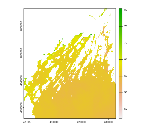
Figure 5

The UTM zones across the continental United
States. From: https://upload.wikimedia.org/wikipedia/commons/8/8d/Utm-zones-USA.svg
Figure 6
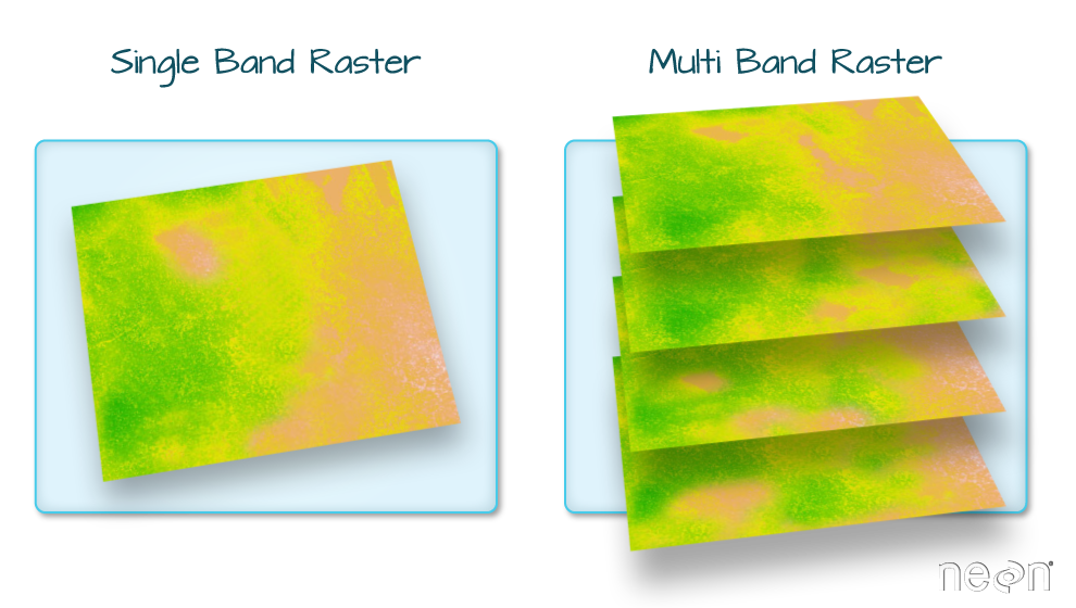
Figure 7
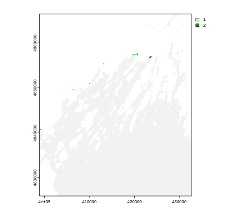
Figure 8
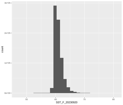
Figure 9
Plot Raster Data
Figure 1
Figure 2
Figure 3
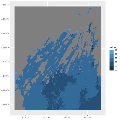
Figure 4
Figure 5

Figure 6
Figure 7
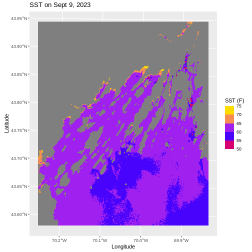
Figure 8
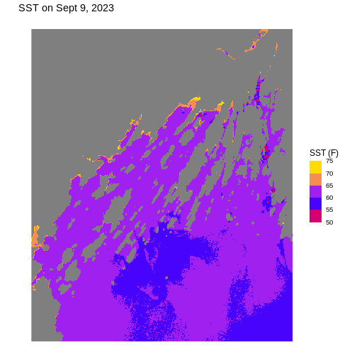
Figure 9
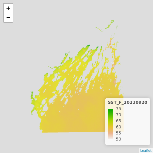
Figure 10
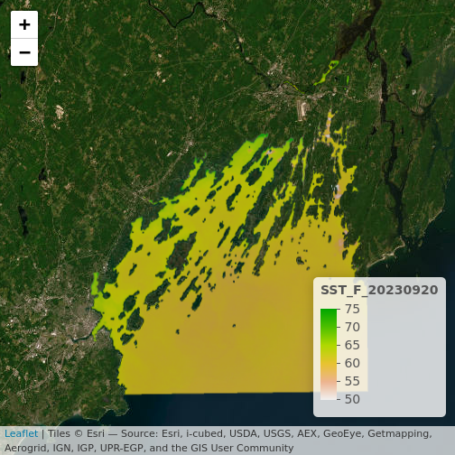
Figure 11
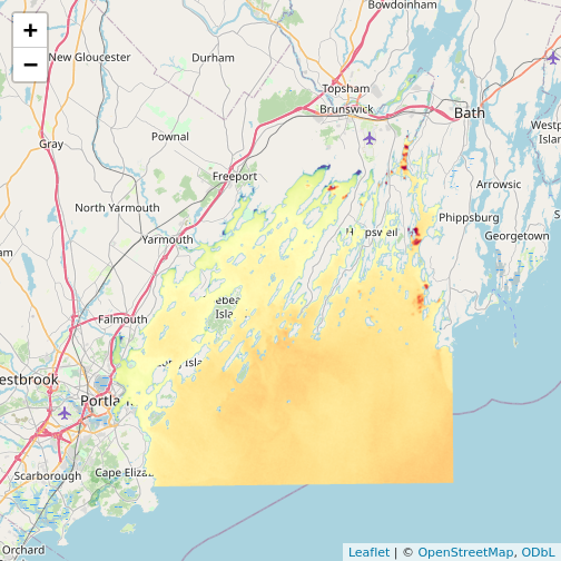
Figure 12
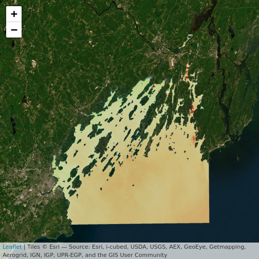
Figure 13
Open and Plot Vector Layers
Figure 1
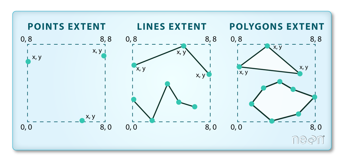
Figure 2
Explore and Plot by Vector Layer Attributes
Figure 1
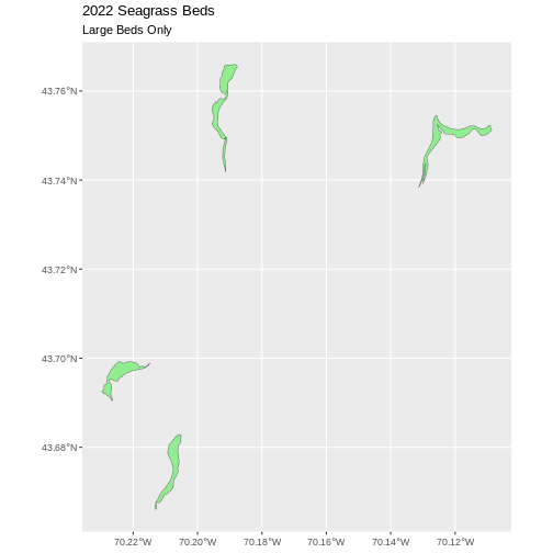
Figure 2
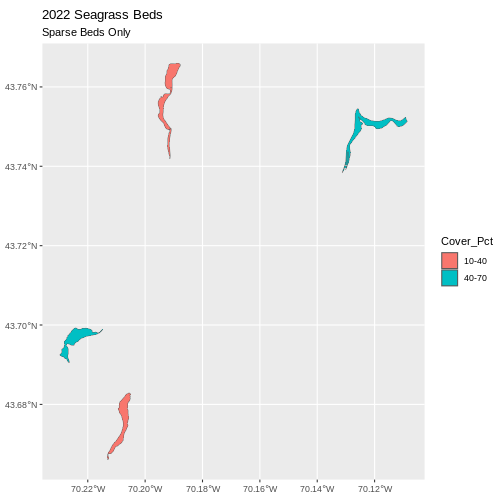
Figure 3
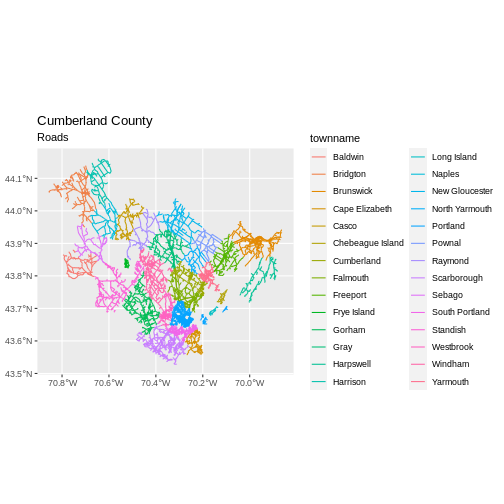
Figure 4
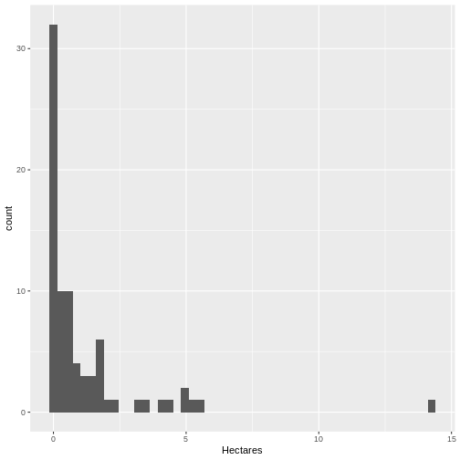
Figure 5
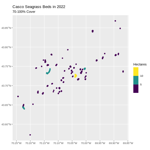
Figure 6
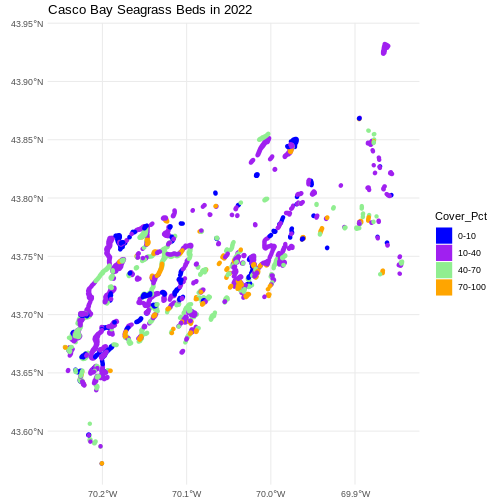
Figure 7
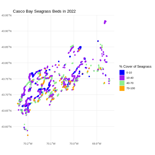
Figure 8
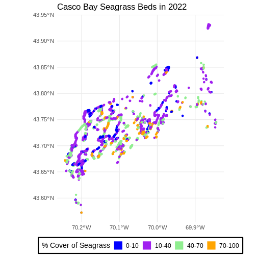
Figure 9
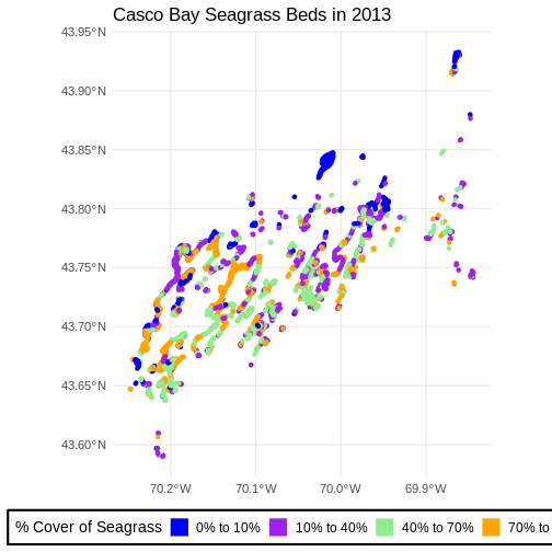
Figure 10
Plot Multiple Vector Layers
Figure 1
Figure 2
Figure 3
Figure 4
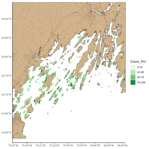
Figure 5
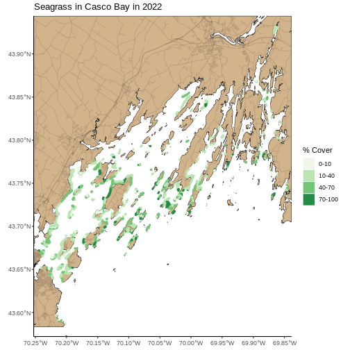
Figure 6
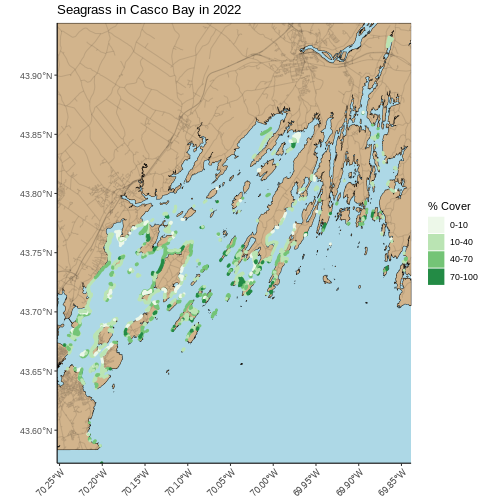
Figure 7
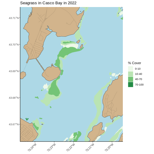
Figure 8
Figure 9
Figure 10
Figure 11
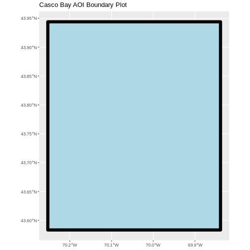
Handling Spatial Projection & CRS
Figure 1
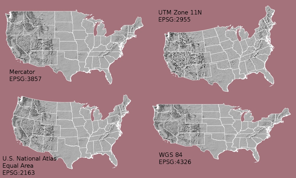
Maps of the United States using data in
different projections. Source: opennews.org, from: https://media.opennews.org/cache/06/37/0637aa2541b31f526ad44f7cb2db7b6c.jpg
Figure 2
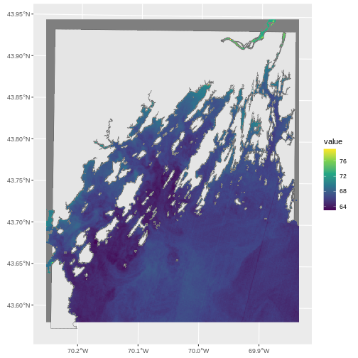
Figure 3
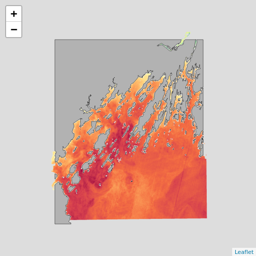
Figure 4
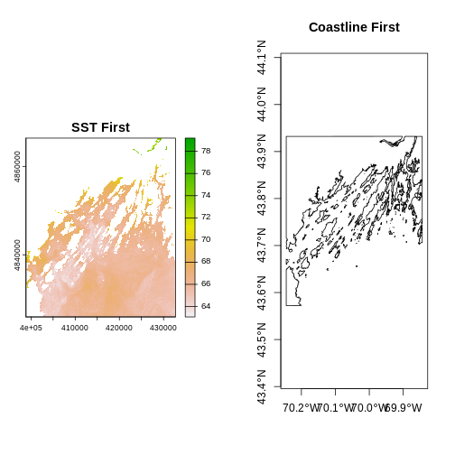
Figure 5
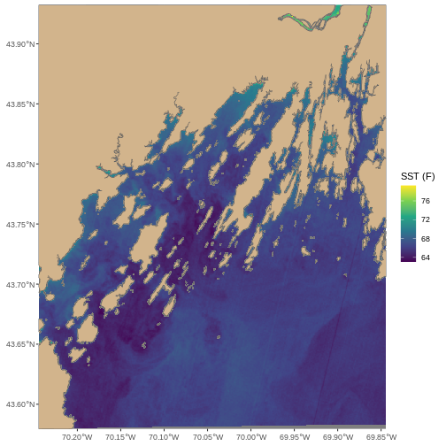
Figure 6
Convert from .csv to a Vector Layer
Figure 1
Figure 2
Figure 3
Extracting Data from Rasters using Vectors
Figure 1
Image Source: National Ecological
Observatory Network (NEON)
Figure 2
Figure 3
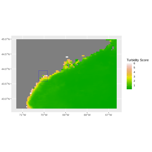
Figure 4
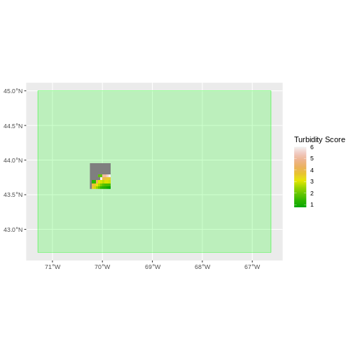
Figure 5
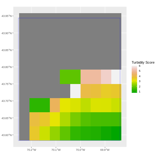
Figure 6
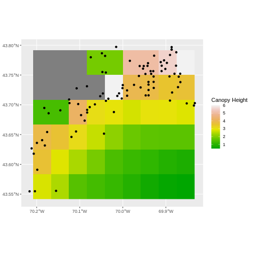
Figure 7
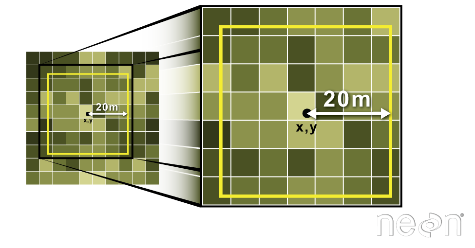 Image Source: National Ecological Observatory Network (NEON)
Figure 8
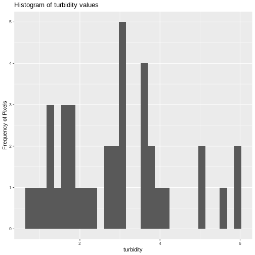
Figure 9
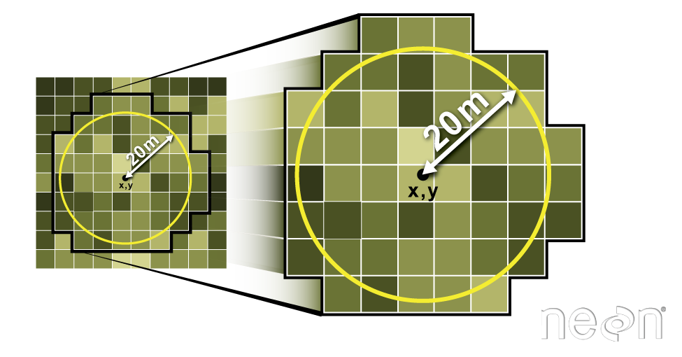 Image Source: National Ecological Observatory Network (NEON)
Figure 10
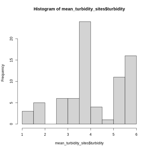
Figure 11
Work with Multi-Band Rasters
Figure 1
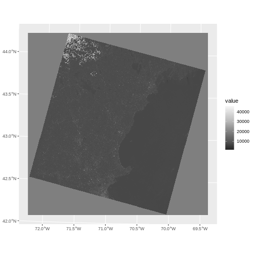
Figure 2
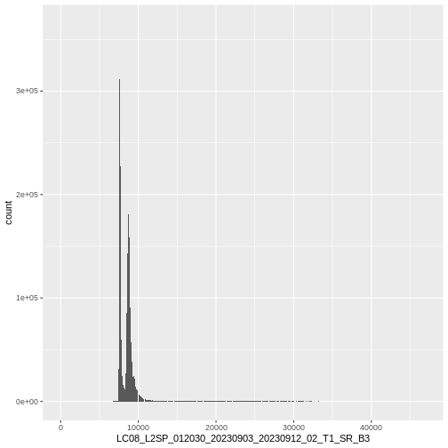
Figure 3
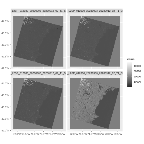
Figure 4
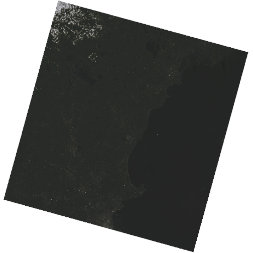
Figure 5
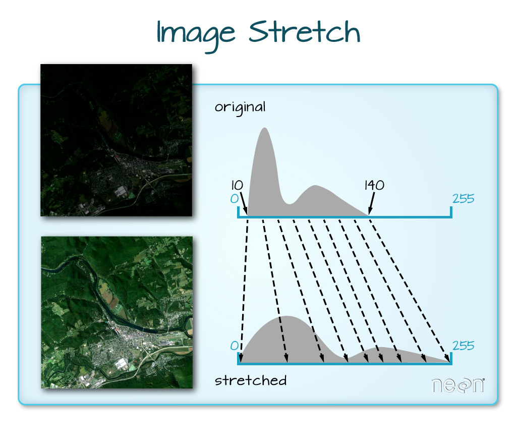
Figure 6
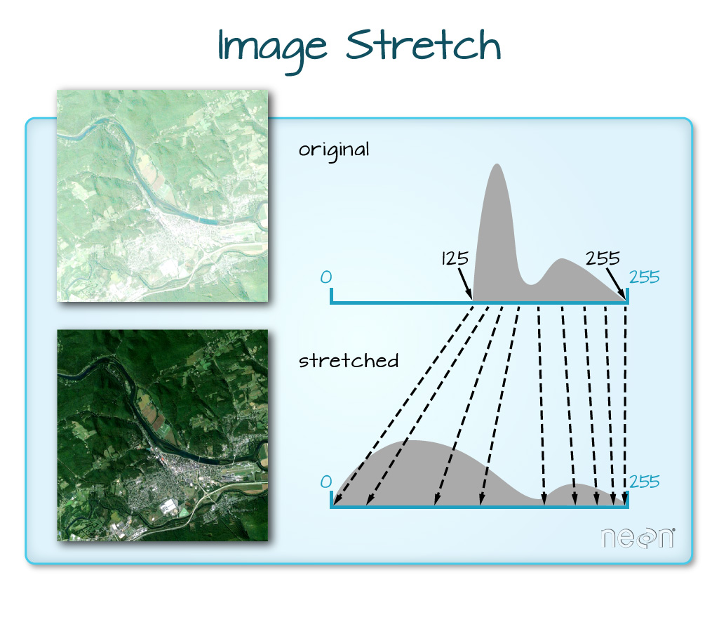
Figure 7
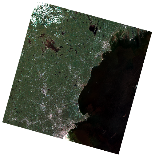
Figure 8
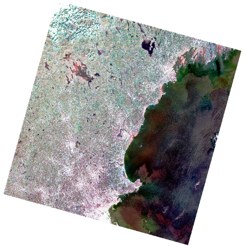
Figure 9
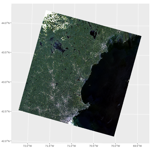
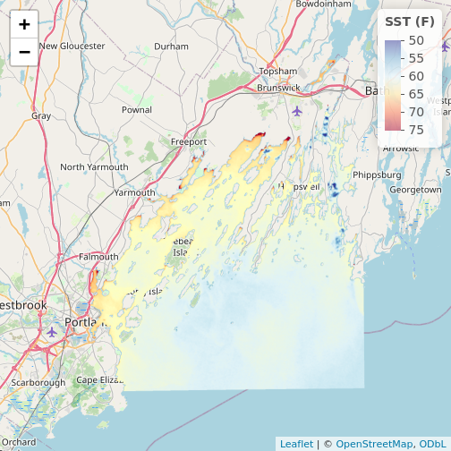
Raster Calculations
Figure 1
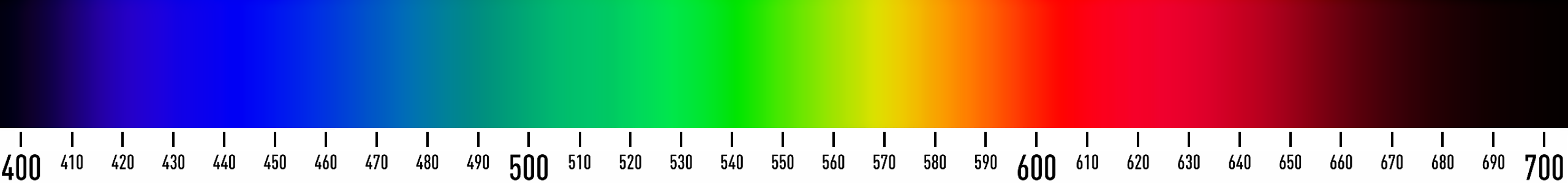
the visible spectrum in nm
Figure 2
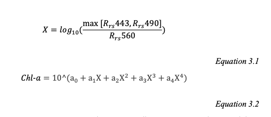
chl eqn
Figure 3
 Let’s see how simple it is
to make these work for us!
Let’s see how simple it is
to make these work for us!
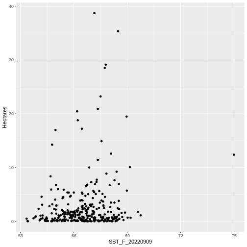
Figure 4

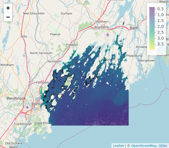
New Hampshire and Southern Maine in Winter
2023
Figure 5
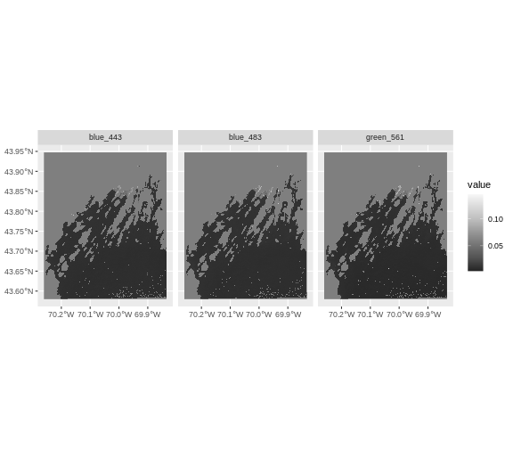
Figure 6
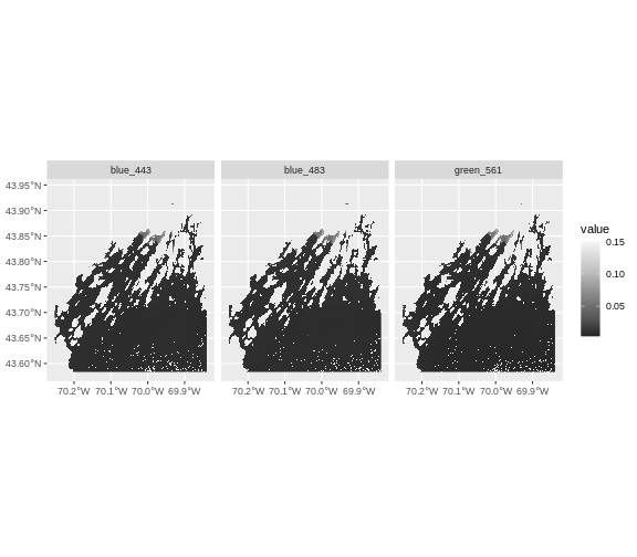
Figure 7
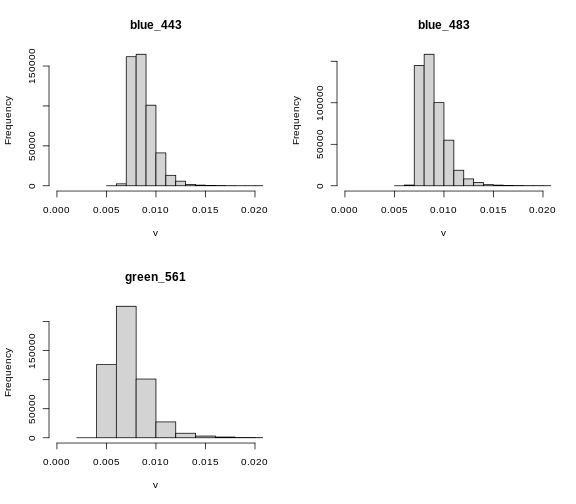
Figure 8
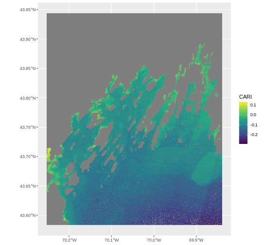
Figure 9
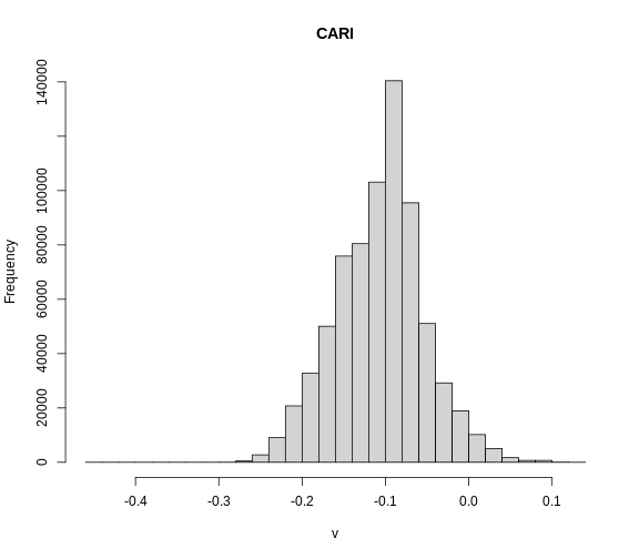
Figure 10
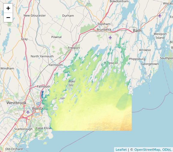
Figure 11
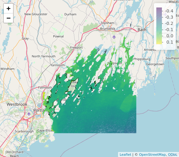
Figure 12
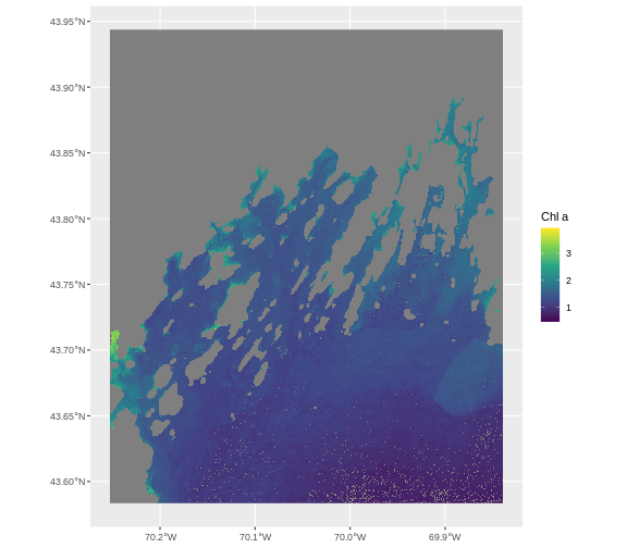
Figure 13